View Function(X,Y)
The View Function(X,Y) option in the View menu is used to graph the surface for a function of X and Y across the X and Y ranges of your choice. This surface graph can be scaled and formatted, its 3D type and view adjusted, and the graph can be printed or copied to the clipboard. You may numerically evaluate the function you have entered, its derivatives, or compute a double integral representing a volume.
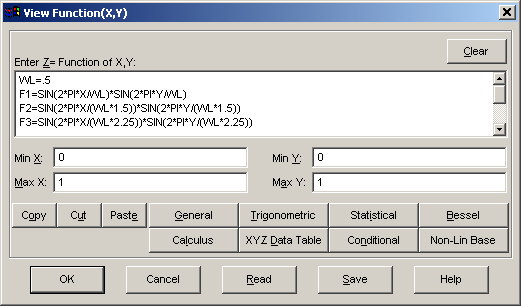
View Function(X,Y) Entry
The View Function(X,Y) entry uses a simple ASCII multiline editor. You can use the Cut, Copy, and Paste items to move text about or to paste in the View Function formula if you placed it into the clipboard via another program. All of the functions and constants available within TableCurve 3D can be accessed via a special Function Insert help. In a View Function, no prefixes are automatically supplied. You may define as many constants as you wish. For example, SQRT2PI=SQRT(2*PI) would be defined on one line and used in subsequent lines. Constant expressions are evaluated once and the numeric result is stored. Any assignment to a variable other than F1-F9 (or #F1-#F9) and Z is assumed to be a constant. Any expression containing X or Y must be assigned either to an F1-F9 expression or to Z. F1-F9 and Z expressions are compiled and are evaluated once for each mesh vertex in the surface plot. The Z expression must always be the last line in the View Function. Here is a simple one-line View Function example:
Z=20+100*(EXP(-((X-55)/20)^2-((Y-45)/18)^2))
In the following multi-line View Function example, S2 defines a constant, F1 defines an expression that is a function of X, F2 defines an expression that is a function of Y, and Z defines the overall View Function:
S2=SQRT(2)
F1=ERFC(-10/S2+LN(X/40)/(10*S2))
F2=ERFC(-12/S2+LN(Y/50)/(12*S2))
Z=20+100*F1*F2
The following example uses the built-in non-linear base functions and the second derivative functions to produce the second derivative peak profile computed from a 3D peak that is Gaussian in the X dimension and Lorentzian in the Y dimension. Note that derivative and integral arguments specify the number of the function being processed rather than the function symbol (1 rather than F1 in DX2, 2 rather than F2 in DY2).
AMPL=100
F1=GAUSSX(AMPL,50,15)
F2=LORY(AMPL,45,12)
Z=DX2(1)*DY2(2)
Ranges
A View Function requires the specification of the initial and final X values and the initial and final Y values.
Saving and Reading View Functions
The Save button is used to save the View Function to disk. For a save to occur, the function must be successfully validated and compiled. A View Function file is saved in a binary format and the default extension is [.VFZ]. The Read item is used to read a View Function from disk. The Clear button simply clears all entry fields.
Validation
A View Function is extensively validated before it is compiled and graphed. If there is a math or parser error, you will be given a clear indication of the error and the cursor will be placed at the location where the validation failed. If successful, the function will be graphed.
View Function Surface Graph
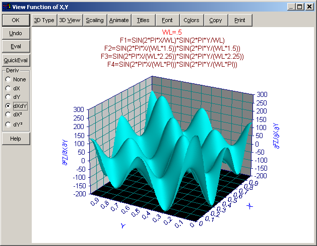
The surface graph will be displayed using a size, position, type, view format, font, and color specific to View Function(X,Y) graphs. These specifications are automatically saved across sessions. You may click within the titles area of the graph to invoke the Custom Titles option, to the left or below the graph to open the Scaling dialog, and within the graph itself to adjust the 3D View.
Undo
Use the Undo item to return to the Function entry screen in order to revise the function, X range, or Y range.
Options
The View Function(X,Y) graph options include:
- Selecting the 3D Graph Type
- Adjusting 3D View Options
- Modifying the Scaling of the graph
- Animating the graph at a succession of view angles
- Setting Custom Graph Titles
- Choosing a Graph Font
- Modifying the Graph Colors
- Copying the graph as a Metafile or Bitmap
- Printing the graph
Evaluation
The Eval item is used to perform a full-featured numeric evaluation of the function.
Real-Time Evaluation
The Quick Eval option offers the means to evaluate the surface at a single x,y, the surface minimum, and the surface maximum.
Partial Derivative Surfaces
In addition to displaying the basic function surface, any of the five first or second partial derivative surfaces can be displayed. These surfaces are computed using numeric derivatives:
- None - the basic function surface
- dX - the first partial derivative with respect to X
- dY- the first partial derivative with respect to Y
- dXdY- the partial derivative with respect to both X and Y
- dX2- the second partial derivative with respect to X
- dY2- the second partial derivative with respect to Y