User-Defined Functions
You may install up to fifteen non-linear User-Defined Functions (UDFs) into TableCurve 3D's equation set at any given time. This User-Defined Functions option in the Process menu is used as the control center for entering, editing, saving, and fitting UDFs. From this UDF dialog, you can work with individual functions or with UDF libraries.
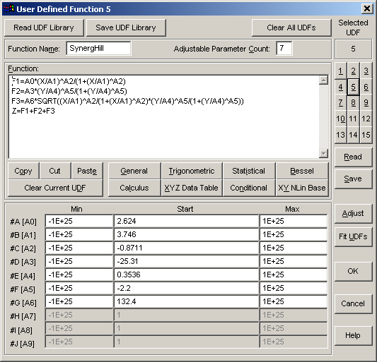
A TableCurve 3D UDF contains all information necessary to fit the function, including the function name, the parameter count, the function's formula, and starting estimates and constraints for each parameter. A special Adjust item allows you to graphically adjust the starting estimates to better assure a successfully converged fit. You may also inspect the partial derivatives for the UDF to find instances of multiple constants, insignificant parameters, and to expose conditions where a fit would be likely to fail.
UDF Selection
The keypad with buttons labeled 1 through 15 is used to select the current UDF. In TableCurve 3D's non-linear equation set, UDF#1 is Equation 2501, UDF#2 is Equation 2502, and UDF#3 through UDF#15 are Equations 2503-2515. UDFs active at any given time need not be sequential and they will remain in the position where you install them, even if lower number UDFs are empty.
Function Name
This name will be used to represent the function in the surface-fit graphs. You will wish to select a name that is meaningful to you.
Coefficient Count
This is the number of adjustable parameters in the UDF model. The UDF must contain the number of parameters entered. If, for example, you enter 4 as the coefficient count, the UDF must contain parameters #A,#B,#C,#D (or A0,A1,A2,A3).
Entering the UDF
The UDF entry uses a simple ASCII multiline editor. You can use the Cut, Copy, and Paste items to move text about or to paste in the UDF formula if you placed it into the clipboard via another program. All of the functions and constants available within TableCurve 3D can be accessed via a special Function Insert help. In a UDF no prefixes are automatically supplied. You may define as many constants as you wish. For example, SQRT2PI=SQRT(2*PI) would be defined on one line and used in subsequent lines. Constant expressions are evaluated once and the numeric result is stored. Any assignment to a variable other than F1-F9 (or #F1-#F9) and Z is assumed to be a constant. Any expression containing X, Y or any of the adjustable parameters #A-#H (or A0-A7) must be assigned either to an F1-F9 expression or to Z. F1-F9 and Z expressions are compiled and are evaluated once for each data point in every iteration. The Z expression must always be the last line in the UDF. Here is a simple UDF example:
S2=SQRT(2) F1=ERFC(-#D/S2+LN(X/#C)/(#D*S2)) F2=ERFC(-#G/S2+LN(Y/#F)/(#G*S2)) Z=#A+0.5*#B*F1+0.5*#E*F2
Using the A0-A7 format, this same UDF would appear as follows:
S2=SQRT(2) F1=ERFC(-A3/S2+LN(X/A2)/(A3*S2)) F2=ERFC(-A6/S2+LN(Y/A5)/(A6*S2)) Z=A0+0.5*A1*F1+0.5*A4*F2
The S2 expression is a constant that is evaluated numerically and stored for use in subsequent expressions. The first function expression, F1, calls the complementary error function with an argument expression containing the third and fourth adjustable parameters and the X variable. The second function expression, F2, performs a similar operation for the sixth and seventh adjustable parameters and the Y variable. The last line is the required Z= function expression. It contains the first, second, and fifth adjustable parameters. The F1, F2, and Z expressions are compiled. In the fit, these expressions are evaluated at the X and Y of every data point for each iteration's particular #A-#G (or A0-A6) adjustable parameters.
Non-Linear Base Functions
Except for the relatively common Gaussian-Log Normal models, TableCurve 3D's built-in non-linear equations use the same base function in both the X and Y dimensions. One common type of UDF will be to use one of the non-linear base functions for the X variable, and a different base function for the Y variable. The following UDF constructs a multiplicative peak function that is Gaussian in the X dimension and Lorentzian in the Y dimension: F1=GAUSSX(A0,A1,A2) F2=LORY(1,A3,A4) Z=F1*F2
Derivatives and Integrals
The following UDF is for fitting the dZ/dXdY cross derivative of this same peak profile, Gaussian in X and Lorentzian in Y:
F1=GAUSSX(A0,A1,A2) F2=LORY(A0,A3,A4) Z=DX(F1)*DY(F2)
Double Integrals
While TableCurve 3D's double integration function is quite fast by comparison with various math programs, fits and surface plots of double integral functions are still likely to be excruciatingly slow all-night affairs. This is true even for a modest number of data points and with a dramatic reduction in mesh counts. You should use the double integral function only in desperation when you are unable to find an analytical solution to the integral and when you are unable to separate the function into f(x) and f(y) components. If you can separate the UDF into f(x) and f(y) components, you can evaluate two single integrals, a process which is orders of magnitude faster than evaluating a double integral. In the first example that follows, the UDF computes the cumulative volume of this Gaussian in X, Lorentzian in Y peak function using the DQIP() double integration function.
Note that non-linear base functions are not used since they are not available for the inner variable of integration $$. In the second example, the function is broken into f(x) and f(y) components with QIP() single integrals. Here the non-linear base functions based upon the variable of integration $ are used. The resulting UDF is orders of magnitude faster in execution than the double integral version. Better still is the third example, which uses the analytic cumulatives built into the program. If you own symbolic math software, or if you enjoy looking up integrals in handbooks, it is strongly suggested that you seek an analytic solution for any integral you need to fit.
For the examples that follow, drawing a minimal 10x10 mesh grid of this double integral UDF required 11.5 minutes on a 486-66 machine. Drawing the two-separate integral UDF on a 10x10 mesh grid required only 5 seconds. The analytic UDF displays in less than 1/4 second. Unlike the integral UDFs, the analytic UDF is normalized so that A0 is equal to the transition height.
F1=A0*EXP(-0.5*(($-A1)/A2)^2)*1/(1+(($$-A3)/A4)^2) Z=DQIP(1,-INF,X,-INF,Y,1E-5) F1=GAUSS$(A0,A1,A2) F2=LOR$(1,A3,A4) F3=QIP(1,-INF,X,1e-5) F4=QIP(2,-INF,Y,1e-5) Z=F3*F4
Z=GCUMX(A0,A1,A2)*LORCUMY(1,A3,A4)
Validation
A UDF is extensively validated before it is compiled. If there is a math or parser error, you will be given a clear indication of the error and the cursor will be placed at the location where the validation failed. If you are having trouble with a UDF, you may save the failed UDF to disk. You can then recall it at some future time in an effort to fix what is wrong.
Starting Estimates and Constraints
You must enter starting estimates for the parameters in the model. Good starting estimates are sometimes necessary for convergence, and usually result in faster non-linear fits. Minimum and maximum constraints are optional. If a parameter violates a constraint that you set, a penalty function is added to the chi-square to attempt to bring the parameter back into a valid range.
Entering Formulas for Estimates and Constraints
You may enter formulas for the estimates and lower and upper limits in UDFs. These enable a UDF to be constructed so as to accommodate widely varying X and Y data ranges. Since these formulas are evaluated sequentially, any given formula can reference a previous estimate. For example, #D can reference #A, #B, or #C, but not #E and higher. More commonly, a UDF estimate formula will reference an XYZ data table constant which TableCurve 3D computes for each data set.
When a UDF contains one or more formulas for the adjustable parameter estimates and limits, it is saved in a binary rather than ASCII form. These UDFs can only be edited inside of TableCurve 3D. The [.UDF] extension is used for both the binary and ASCII formats.
Reading a UDF
Use the Read button to read a UDF from disk. The UDF will be read into the current UDF position, replacing any UDF that might currently be in this same position. You may read any UDF into any of the 15 available positions, even if lower numbered positions are empty. This option will read both the ASCII format UDFs and the binary format UDFs containing one or more formulas for estimates or constraints. It is recommended that UDFs be created only within the program.
Clearing a UDF
Use the Clear Current UDF button to immediately free the currently selected UDF from memory and to reset the UDF entry screen.
Saving a UDF
Use the Save button to save a UDF to disk. If the estimates and constraints are numeric, the UDF is saved in an ASCII format with a [UDF] extension. If formulas are present, the UDF is saved in a binary format that requires approximately 4K of disk space. A UDF is always validated before a Save is made. If the validation fails, you are given an option to save the UDF even though it contains an error. You can then recall it at some future time in an effort to repair what is wrong.
Saving a UDF Library
To make it easy to work with up to 15 user functions, any set of installed UDFs can be saved as a user function library. UDF positions are preserved as you enter them and installation of empty UDF positions are permitted. UDF libraries are saved as binary [UDL] files, whether or not estimates contain formulas. In a UDF library, each UDF consumes about 4K, so a full 15 UDF set will require about 60K disk space. To save the current set of UDFs to a library, use the Save UDF Library button. For maximum flexibility, you may wish to save individual UDFs as separate files in addition to having them in libraries. If you choose to keep UDFs only in libraries, you can save out individual UDF components simply by reading the UDL library, selecting the UDF of interest, and then using the individual Save option.
Reading a UDF Library
To read the user functions within a TableCurve 3D UDF library, use the Read UDF Library button. This will install and validate all of the UDFs in the UDL library. If a validation fails, you are notified of such and that specific function is not installed. To extract a UDF from a library, use this option, select the UDF desired, and then use the individual Save option to create the UDF file.
Clearing All UDFs
To clear all of the currently installed UDFs from memory and to clear the current entry screen, use the Clear All UDFs button. You must confirm this option before the UDFs are freed. Note that it is not necessary to clear the existing UDFs when reading a UDF library since all current UDFs are cleared prior to this read operation.
Immediate Fit
Use the Fit UDFs button to immediately fit the UDFs. This is the same as the Surface Fit User Functions item in the Process menu. Note that this option fits all installed UDFs. The fitting only occurs if the current UDF is successfully validated.
Parameter Contribution Warning
Even with a successful UDF compilation, you may still get the warning Parameter n Makes Less Than.1% Fractional Contribution to Equation in Range of Data. Adjustment is Recommended. TableCurve 3D determines the minimum and maximum partial derivative for each parameter. This range of partial derivative is multiplied by the current estimate for that parameter and then compared to the overall Z-data range. If a parameter does not make at least a.1% contribution relative to the Z-data range, this warning is given.
This is often a good indicator that the fit will fail because of poor starting estimates. It may also indicate a poorly designed model that contains a parameter that minimally impacts the equation in the X,Y-range of the data. When this message occurs, it is recommended that you use the Adjust procedure to refine the estimates, and if necessary, the Adjust procedure's Derivatives option to see if an insignificant parameter is present.
If You are Uncertain of Starting Estimates
When working with a new or exploratory model, you may not know what values constitute good starting estimates. In such a case, for each parameter you are uncertain of, simply enter 1.0 for the starting estimate (or some other value for which the UDF is defined). If you achieve a successful compile but get the parameter contribution warning, use the Adjust item to graphically set the estimates.
If you do not get the parameter contribution warning, there is a good chance the fitting algorithm may successfully converge. There is no harm in letting the fitting algorithm do the work. Use the Fit UDFs option to fit only the UDFs. If you are successful, you may wish to take note of the successful parameters and modify the UDF accordingly. If the fit fails, you must return to the UDF screen and use the Adjust feature to graphically set the starting estimates to better reflect the data.
Alternatively, you may want to use the Find and Update feature in the Adjust procedure. This performs a limited convergence fit with a subset of the data and automatically places the parameters in the starting estimate fields. In rare cases, this reduced data set fit can wander off into oblivion producing meaningless estimates. If this occurs simply use the Reset button or Cancel out of the Adjust dialog to discard the modified estimates. In most cases, the Find and Update should produce excellent estimates. If there is a revision of a parameter initially entered as a formula in the main UDF dialog, either by manual adjustment or via the Find and Update option, you must confirm that the original formula for the estimate is to be replaced with the new numeric value. Note that any save operations occurring after this replacement will use this numeric value.
Graphical Adjustment of Starting Estimates
Use the Adjust item to open a graph of the data and the UDF surface. Do not be surprised if you do not see the UDF surface at first. If the estimates are too far off, it is possible that no part of the UDF surface will be anywhere within the field of the X,Y,Z data.
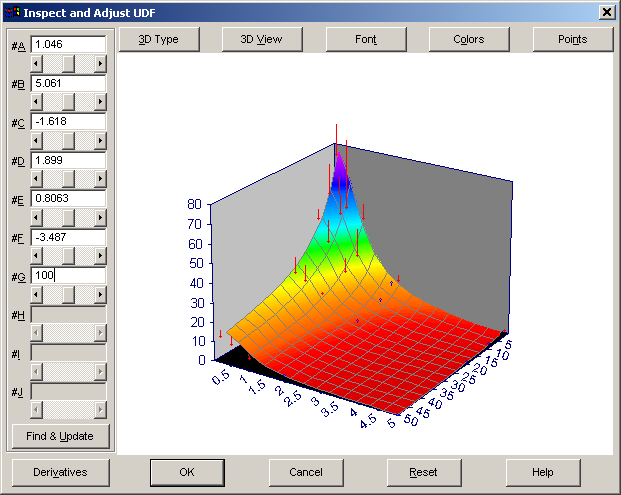
The goal of graphical adjustment is to set the parameters so that the UDF starts to approximate the data. You may adjust each parameter with the scrollbar or you may enter the actual value. If you enter an actual value, there will be a brief delay before the screen is updated, allowing you to complete your entry.
For each parameter that has user-specified minimum and maximum constraints, as opposed to the defaults, the scrollbar adjustment will range from this minimum to maximum in 100 steps.
If such constraints are absent, the scrollbar's sensitivity will depend on computed partial derivatives. The partial derivatives are updated with each value entered. If you enter a value for which the partial derivative range is very nearly zero, or if such is true when you begin, the scroll bar adjustment may produce very large jumps. In this case you must enter a value that brings the UDF back into range.
Find and Update
The Find and Update button in the Adjust screen initiates a low convergence fit using a subset of the current data table. The results of this very rapid pre-fit are automatically placed within the starting estimate fields. While this is often a very attractive means for refining the starting estimates, the algorithm is as vulnerable to local minima as the main non-linear fitting engine. In rare cases, this reduced data set fit can wander off into oblivion producing meaningless estimates. If this occurs simply use the Reset button or Cancel out of the Adjust dialog to discard the modified estimates.
UDF Failures
The two most common causes of UDF failures are having the UDF produce essentially a constant value across the X and Y ranges of the data, or to have a parameter set at such a value, that its impact totally masks the impact of X and Y varying across the range of the data.
As you adjust the starting estimates graphically, the UDF is being updated. When you return to the UDF screen, the estimates will reflect those set in the graphical procedure. By careful attention in the Adjust feature, no valid UDF should fail to produce the intended fit.
Inspecting Partial Derivatives
From the graphical UDF Adjustment screen, you can choose the Derivatives option. This displays a similar set of adjustment controls except instead of seeing a graph, you see a table of partial derivative information.
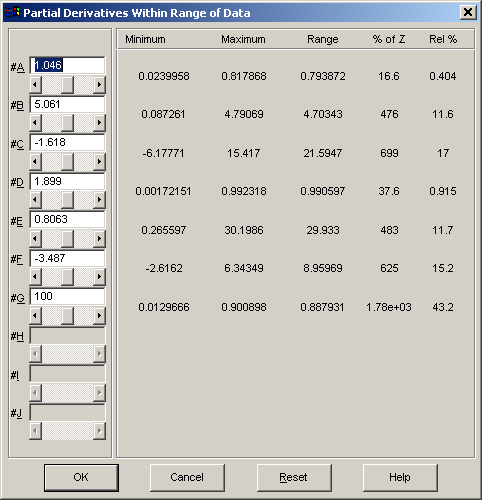
The % of Z column consists of the % of the Z data range represented by the range of the partial derivative multiplied by the estimate. The last column reports a relative percent based on all non-constant parameters, and these sum to 100%.
The fitting algorithm relies on changes in partial derivatives to guide the revisions in the parameters that occur with each iteration. If a partial derivative is constant, then it should have a value of 1.0, meaning that it is a true constant in the expression. If you see two constants, then at least one of these parameters should be removed. If you find that across wide adjustments of a given parameter there is no significant contribution to the Z-range of the data, whereas the others are making such a contribution, you should seriously question whether this parameter belongs in your model.
Note that you can set the estimate of a given parameter so far out of range that no legitimate partial derivatives are found for any parameter in the X,Y-range of the data.