Estimate Gridded Data

The Estimate Gridded Data option in the Non-Parametric menu is intended for interpolating and extrapolating data that exist in a regular grid format. A regular grid has distinct, though not necessarily uniformly spaced, elements.

Non-gridded data can be processed directly with this procedure (the option automatically invokes the Renka I procedure to interpolate the incomplete elements in a grid formed by the unique x and y values in the input data). For a greater flexibility in interpolation algorithm, the Fill Sparse Grid procedure can be used. For complete control of the algorithm and grid dimensions, the Interpolate to Uniform Grid option is available.

In general, the Estimate Scattered Data option is recommended when the data lack this regular grid format.

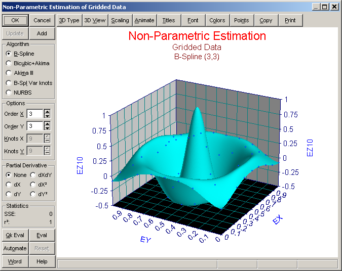
This option creates an output object as opposed to an XYZ data object when added to the notebook in the TableCurve 3D explorer. If needed, XYZ data files can be created in the Eval option and subsequently added as data sources.

To smooth data prior to non-parametric fitting, use the Smooth Loess or Smooth NURBS option in the Table menu.

Algorithms

Five different algorithms are available:

• B-Spline
• Bicubic+Akima
• Akima III
• B-Spl Var knots
• NURBS

Interpolation and Smoothing

The first three algorithms are strictly interpolation routines whose surfaces pass exactly through the data. The B-Spl Var knots and NURBS algorithms are smoothing procedures. These are furnished mainly so that smoothed higher order derivatives can be explored directly.

Note that the B-Spl Var knots procedure is not recommended for data smoothing. For such smoothing, the Loess smoothing procedure in the Smooth Data option is recommended.

Smoothness and Continuity of Partial Derivatives

A biquadratic (order 2/2) spline offers a smooth surface and continuous but not smooth first partial derivatives.
A bicubic (order 3/3) spline offers a smooth surface, smooth first partial derivatives, and continuous second derivatives.
A biquartic (order 4/4) spline offers a smooth surface, smooth first and second partial derivatives, and continuous third derivatives.
A biquintic (order 5/5) spline offers a smooth surface, smooth first, second, and third partial derivatives, and continuous fourth derivatives.

The Bicubic+Akima and Akima III options have the smoothness and continuity of a bicubic spline.

Smoothness and Rounding at Nodes

A higher order interpolant will introduce more rounding at the nodes than a lower order one. As such a higher order surface can be considered "smoother" than a lower order one even though both produce a smooth continuous surface that passes exactly through the data.

Extrapolation

The Akima III, Bicubic+Akima, and NURBS (bicubic only) options offer extrapolation. In these cases, there will be a smooth transition between the interpolated and extrapolated regions of the surface. The first order partial surfaces will be continuous at this transition, although smoothness will be lacking at this boundary.

Surface Type

The Partial Derivative option allows for the following surfaces:

• None - the actual interpolant
• dX - the first partial derivative with respect to X
• dY- the first partial derivative with respect to Y
• dXdY- the partial derivative with respect to both X and Y
• dX2- the second partial derivative with respect to X
• dY2- the second partial derivative with respect to Y

Note that the higher order derivative surfaces will not be continuous with biquadratic (order 2/2) splines. Smoothness in the second order derivative surfaces requires a biquartic (order 4/4) spline.

Statistics

For the B-Spl Var knots and NURBS procedures, where smoothing occurs, the surface will not pass exactly through the data. To enable the results of a non-parametric fit to be compared with parametric fits, a squared sum of residuals (SSE) and a coefficient of determination (r2) are displayed. For the exact interpolation procedures, the SSE will be 0 and the r2 will be 1.

Evaluation

The Eval button is used to open a full featured evaluation procedure. Individual function, partial derivative, roots, and volumes can be computed. This option can also be used to generate a table based upon a uniform grid or input XY data from any of TableCurve 3D's supported formats.

Note that this Generate Table option in the Evaluation is the only way to convert data to a partial derivative for subsequent parametric fitting.

Real-Time Evaluation

The Quick Eval option offers the means to evaluate a few basic properties of a surface in a real time as algorithms and settings are changed. Simply enter an X and Y value in order to have a Z computed automatically with each change in the surface. Since optimizations are such an important part of surface science, the Surface Min and Surface Max check boxes allow for the display the X,Y,Z coordinates of the minimum and maximum of the surface. These are found by a two dimensional minimization algorithm that seeks 1E-8 fractional precision.

Graph Controls

This option offers the common TableCurve 3D graph controls:

• 3D Type
• 3D View
• Scaling
• Animate
• Titles
• Font
• Colors
• Points
• Copy
• Print

Add

The Add button adds an Estimate Gridded Data object to the currently selected XYZ data object in the TableCurve 3D explorer. This is an output object that can be added to any item containing XYZ data, although data on an XY grid are recommended.

Update

If an Estimate Gridded Data item is currently selected and the main graph is clicked, the Update button will be enabled. This updates the non-parametric fit with the current settings as well as updating all graph customizations.

Batch Automation

The Automate button activates the TableCurve 3D Automation facility. This allows unattended processing of large numbers of data sets. The data sets can be consolidated in an Excel file or acquired using a DLL. The graphs and reports can be exported to a Microsoft Word/RTF file, while the processed data can be exported to an Excel 95 or Excel 97/2000/XP file.

If an Automation session is in progress, the Reset button can be used to terminate the automated processing.

MS Word/RTF Export

The Word button is used to save the current graph to either a MS Word file or a portable RTF (Rich Text Format) file. The graph is inserted into the file as a Windows metafile.

Preserving the Current Interpolation Settings

Exit with OK to update the procedure's settings. These values will be reflected the next time the procedure is entered. To discard the current settings, close the procedure with the Cancel button. Note that the Add or Update options must be invoked before closing the dialog in order for the non-parametric output to be added to the current notebook.