Numerical Methods

Linear Fitting

All TableCurve 3D linear fitting algorithms use 80 bit floating point math. This is the full 19-digit precision of Intel floating-point hardware. This highest precision was chosen because most matrix operations are highly susceptible to precision losses and roundoff errors. Using software other than TableCurve 3D, even with the same procedures, you may find different fitted coefficient values for a given equation if such programs use 32 or 64 bit precision.

All of TableCurve 3D’s linearly fitted equations use a single step Gaussian Elimination matrix solution method for the coefficients and a single step Gauss-Jordan matrix inversion for the standard errors and confidence intervals.

Optionally, you may activate an auto-SVD option which performs an additional SVD fit when the design matrix reciprocal condition number is less than 5E-14. If the SVD fit produces a smaller sum of squared residuals, the results of this fit will replace the Gaussian Elimination results. When the coefficient values have been determined by SVD, the standard errors and confidence intervals are determined by an SVD inverse. Note that the auto-SVD option increases fitting time. For a discussion of the auto-SVD option, please refer to Chapter 10.

For more information on linear fitting algorithms, the following references may be of interest:

Bevington, Philip R. 1969, Data Reduction and Error Analysis for the Physical Sciences (New York: McGraw Hill)
Dongara, J.J. et al. 1979, LINPACK User’s Guide (Philadelphia: Society for Industrial and Applied Mathematics)
Press, William H. et al. 1988, Numerical Recipes in C; The Art of Scientific Computing (Cambridge,UK: Cambridge University Press)

Selective Subset Algorithm

TableCurve 3D’s Selective Subset algorithm was designed specifically for the product and is not based upon any published algorithm. Its intent is to reproduce the results of algorithms known as “Best Subset” and “All Possible Subsets”, but to do so in a far more rapid manner.

TableCurve 3D’s Selective Subset algorithm seeks to select from all possible combinations of 21 X-basis functions and 21 Y-basis functions, those equations having up to nine coefficients which produce the best least-squares fits.

In a test case, a nine term-count limited “Best Subset” algorithm similar to that found in certain statistics packages required over 12 hours to fit the 42 basis functions. TableCurve 3D’s Selective Subset algorithm, on the other hand, produced the same best equations in 30 seconds.

The premise of the Selective Subset algorithm is that it is possible to selectively discard basis functions as the term count increases. In other words, all 42 basis functions are used for the simple three coefficient fits, but this number can be successively decreased with higher term count. By doing so, the number of permutations is dramatically reduced at each step.

The Selective Subset algorithm must necessarily do all three parameter fits first, then the four parameter, and so on through to the nine parameter fits. In each level, a merit function is assigned to each basis function. Those least contributing to the various fits are discarded before the next level begins.

This is how TableCurve 3D can select from over 450,000,000 equations and fit only 36,000. And yet, even with less than 0.01% of the possible equations actually fitted, the results can be identical or nearly so to having fitted the whole set.

In defense of “Best Subset” and “All Possible Subset” algorithms, it is important to note that their purpose is primarily not to deal with multiple basis functions of one or two variables, but to deal with a large number of independent variables. In such instances, it is quite appropriate to fit every possible permutation to insure each independent variable’s impact is fully appraised.

In TableCurve 3D, the Selective Subset equations also include ln(Z) and 1/Z transforms. If the best of the three term count transformed subset equations is poorer than the worst of the saved standard Z equations, the fits are terminated early without progressing to higher term counts.

Non-Linear Fitting

Non-linear equations are those which cannot be solved in a single step solution of a matrix, but must be managed in an iterative fashion. As such non-linear fitting is a much slower process and one that often requires starting estimates in order to initiate the fitting.

TableCurve 3D’s non-linear fitting engine is a 64-bit Levenburg- Marquardt algorithm that uses the Gauss-Jordan procedure for the matrix inverse required in each iteration. In non-linear fitting, the parameters are iteratively adjusted to minimize a goodness of fit merit function usually referred to as c2. If the algorithm is fully successful, a true global minimum (the true least-squares fit) is achieved.

Since the Levenburg-Marquardt method’s minimization procedure requires the partial derivatives with respect to the parameters, TableCurve 3D uses analytic derivatives for the 168 built-in functions for the highest precision and the most rapid fitting and convergence.

The Levenburg-Marquardt algorithm requires starting estimates for the adjustable parameters. For the 168 built-in non-linear equations, these are automatically supplied by the pre-scan procedure.

The non-linear fitting algorithm can be configured for the maximum number of iterations as well as to specify a convergence criteria. TableCurve 3D deems the algorithm converged when the r² coefficient of determination is unchanging in the significant digit specified for five consecutive iterations. The fitting engine can also be interrupted to terminate a non-linear fit that is going nowhere, but is still slowly changing in the r² merit function.

TableCurve 3D’s user-defined functions are a part of the non-linear fitting engine. Here the starting estimates must be supplied by the user. User-functions are compiled and fitted in 64 bit precision, using numeric derivatives. Successful convergence may well depend upon the quality of the starting estimates.

For more information on the Levenburg-Marquardt non-linear fitting algorithm, see the Bevington and Press references previously given.

Integration, Minimization, and Root-Finding Algorithms

TableCurve 3D uses a double integration Gaussian Quadrature method for computing volumes beneath surfaces. The Quadrature procedure’s convergence is targeted for eight significant figures. In the Evaluation option, the precision actually achieved is reported.

In the AI() and AIP() integration functions used primarily for UDFs, a Gaussian Quadrature procedure is first used. If the target precision is not achieved, a Romberg procedure is then attempted. If neither algorithm achieves the target precision, the UDF will use the value from the procedure that came closest.

A two-dimensional version of Powell’s direction set minimization procedure is used for determining the minima and maxima of the fitted equation.

The root-finding routine in TableCurve 3D is a multi-partition bisection procedure.

For more information on these methods, please refer to the Bevington and Press references.

Statistical

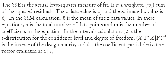
Sum of Squares due to Error (Sum of Residuals Squared)

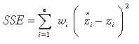
Sum of Squares about Mean

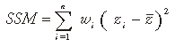
Coefficient of Determination

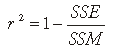
Degree of Freedom

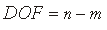
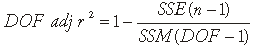
Degree of Freedom Adjusted r2

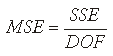
Mean Square Error

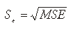
Fit Standard Error (Root MSE)

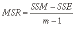
Mean Square Regression

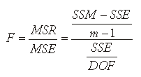
F-statistic

Confidence Interval

Prediction Interval