Robust Fitting
 By selecting a robust minimization procedure in the Surface-Fit Preferences option, robust fitting can be done for any of TableCurve 3D's non-linear equations, including UDFs.
 The Process menu also includes a Surface-Fit Robust Plane option which fits the simple plane by least squares and by all three of TableCurve 3D's robust minimizations.
A Robust Fitting Example
Least-Squares and Removing Outliers
The statistics reported for a least-squares fit assume that the residuals follow a Gaussian or a normal distribution. The points that lie outside ± 3 standard errors, which by default are red, should occur on the average only once every 370 points. It is not uncommon to see a higher frequency of points outside 3 standard errors. When such outliers occur, one solution is to simply exclude these points and refit. The exclusion will be based on the residuals for a specific equation, so you will want to select your desired equation before isolating the outliers, excluding them, and refitting.
In some instances, this removal of outliers isn’t at all straightforward. This exclusion based on points outside ± 3 or ± 2 SE uses an assumption of normally-distributed or Gaussian errors. Life isn’t so simple when errors are far from Gaussian or unevenly distributed. Consider the following least-squares fit of a simple plane data set:
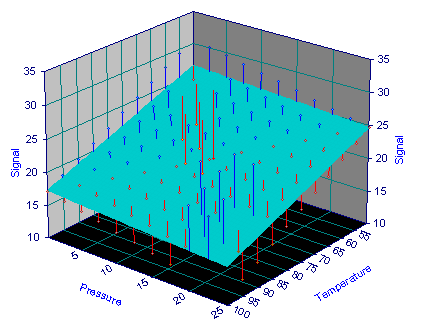
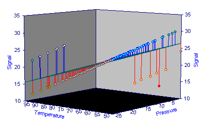
In the second graph, the view angles have been adjusted so that the points in the plane appear as a line. Note that the impact of the outliers present in this data set is to shift the fitted surface significantly away from the bulk of the data defining the plane.
One solution is to exclude the outliers and refit. The points that lie outside ± 3 SE (colored red by default) should always be excluded, and probably those outside ± 2 SE (colored yellow by default). Even doing so, however, note that not all of the outliers would be removed.
Maximum Likelihood Estimation
Removing outliers is difficult, tedious, and can readily introduce bias. A better approach is to use a robust or a maximum likelihood minimization that ignores the influence of outliers.
In this example, there is a readily apparent sense that it is “likely” the surface should shift a great deal more toward the bulk of the data defining the plane. What we seek then is a method that automatically offers a more robust fit, one that is far less sensitive to data points which are unlikely to be valid. With least squares, outliers have far more influence in the overall goodness of fit merit function than than those observations that are more accurate.
TableCurve 3D’s non-linear engine offers built-in three robust maximum likelihood fitting algorithms. The following surface fit results from using TableCurve 3D's Lorentzian minimization:
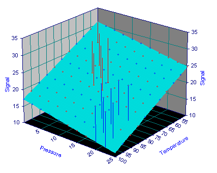
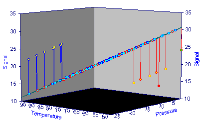
The effects of the outliers have been virtually eliminated.
Least-Squares and Robust Minimizations
TableCurve 3D’s non-linear fitting offers three robust methods that can be used instead of least squares. These methods are built directly into the non-linear engine enabling all non-linear functions, including UDFs, to be fitted by a robust method.
While TableCurve 3D classifies these three methods as having low, medium, and high levels of robust performance, it should be noted that least absolute deviation, the least robust of TableCurve 3D’s methods, is still very effective in minimizing the influence of outliers.
Least-Squares
Least-squares fitting involves the minimization of the weighted sum of the squared residuals.
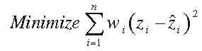
There are two instances where this minimization produces a less than satisfactory fit.
The first is where significant outliers are present. In this case, the square of the residuals of these outlier points may, within a given region, significantly shift the fitted surface away from the bulk of the data.
The other instance is when the Z data values span more than several orders of magnitude. The squared residuals of the largest valued Z-points can overwhelm the influence of the squared residuals of the smallest Z-valued points, causing the smallest Z-value points to either be poorly fitted or not fitted at all. Data that requires a logarithmic Z-scale to see all of the points may be a good candidate for robust fitting, especially if four or more major log divisions are present.
Least Absolute Deviation
The essence of robust fitting is to use a minimization that is less influenced by outliers and the dynamic range of the Z-variable. Instead of minimizing the weighted sum of the squares of the residuals, an obvious alternative is the minimization of the weighted sum of the absolute value of the residuals.
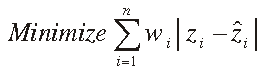
This is probably the best known robust method, though not necessarily the best, and is usually designated as least absolute deviation. Of TableCurve 3D's three robust methods, least absolute deviation is usually the least powerful in terms of managing outliers.
Lorentzian Minimization
The intermediate method in terms of power of robustness is a Lorentzian minimization.
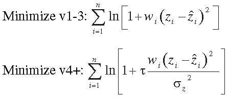
This merit function scales the squared residual by the variance in the Z variable and adds tau, a term that controls the width of the applied Lorentzian, and thus the power of the robustness.
If you are uncertain of which robust method to use, we strongly recommend this Lorentzian minimization. It is very effective when you have noisy data with outliers or if your data span many orders of magnitude in Z. These fits also tend to converge as rapidly as the least absolute deviation minimization.
Pearson VII Limit Minimization
This is the most robust of the three methods.
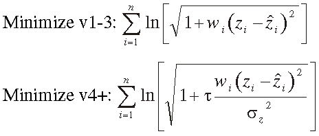
This merit function also scales the squared residual by the variance in the Z variable and also adds tau, a term that controls the width of the applied Pearson VII limit model, and thus the power of the robustness.
With this method, outliers tend to have almost no impact on the fitted surface. This minimization represents an extreme one that can manage very wild errors.
Scale Invariant Fitting
By their nature, the least squares and least absolute deviations are scale invariant. The derivative of the merit function defines the "influence curve" in maximum likelihood fitting. If m is the magnitude of a given residual, then the influence curve for least squares is proportional to 2m, linearly increasing, and for least absolute deviation is 1, a constant. In neither case does the assigned width of the assumed error distribution impact the fitting since the influence curve is either linear or constant. If the Z values are multiplied by a factor of 10, or 0.1, or any scalar, the merit function scales accordingly and the same overall fit is realized. Parameters which do not depend on the magnitude of Z remain unchanged.
Because the residual is contained within a logarithm expression, this is not true of the unscaled Lorentzian or Pearson VII Limit minimizations used in TableCurve 3D releases v3 and prior. The influence curve of the Lorentzian and Pearson VII Limit minimizations is not linear. If the Z values are multiplied by any scalar, a different overall fit occurs. Parameters which do not depend on the magnitude of Z have different values.
From release 4 onward, TableCurve 3D uses a scale invariant form for the Lorentzian and Pearson VII Limit minimizations. These robust minimizations will now produce the same overall fit when the Z values are multiplied by any scalar value. In these forms, the residuals are scaled by the variance in the Z data values, and an additional parameter, tau, is added. This controls the width of the underlying distribution. Unlike least squares and least absolute deviation where the width of the underlying assumed distribution is unimportant because of the linear or constant influence curves, the width of the underlying or assumed distribution for the Lorentzian and Pearson VII Limit minimizations is critical. Tau fixes how the distribution of residuals are placed across this non-linear influence curve, and hence impacts the power of the robustness.
The tau for the Lorentzian has been fixed at 100 and the tau for the Pearson VII Limit is fixed at 1000. These values were determined empirically as a balance between the power of robustness and the sensitivity to local minima in the starting estimates.
Starting Estimate Sensitivity
Robust fitting is more sensitive to starting estimates than least-squares. If the power of robustness is too great and the initial estimates define a surface that passes close to outliers but not to the main body of the data, there is a risk of these outliers being seen as the "correct" surface by the fitting algorithm. The greater the power of robustness, the more a few points very close to the surface as defined by starting estimates can dictate the final position of the fit.
If the expected results for a Lorentzian or Pearson VII Limit minimization are not realized, you may need to set UDF starting estimates closer to the true surface and away from any surface formed by outliers that may be present. If this arises for a built in model, you will need to generate a UDF and manually set the necessary initial estimates.
The Pearson VII limit minimization has a greater starting estimate sensitivity than the Lorentzian. This is why there may be instances where the Lorentzian fitting iterates to the desired surface, but the Pearson VII Limit produces an inferior fit.
Error Distributions
Each of the various minimization formulas corresponds with a maximum likelihood probability distribution:
- When a least squares minimization is made, a maximum likelihood fit is achieved only when the errors follow a Gaussian or normal probability density.
- When a least absolute deviation minimization is made, a maximum likelihood fit is achieved only when the errors follow a double sided exponential probability density.
- When a Lorentzian minimization is made, a maximum likelihood fit is achieved only when the errors follow a Lorentzian probability density.
- When a Pearson VII Limit minimization is made, a maximum likelihood fit is achieved only when the errors follow a Pearson VII width=0.5 probability density.
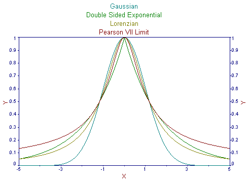
Note that nothing enforces a maximum likelihood result. It is a concept that is subject to highly restrictive assumptions. While least-squares fits often produce a normal distribution of errors, and can thus be regarded as producing the maximum likelihood estimates for parameters, this is not likely to occur in practice for any of the robust minimizations. At best, the robust fits may coarsely approach the maximum likelihood estimates.
A least-squares fit can be made for any data set and all manner of residuals distributions can result. The same is true for any of the robust minimizations. That a fit fails to produce its corresponding maximum likelihood error distribution doesn't invalidate the fit, but it should call into suspicion the standard errors and confidence limit statistics which assume such an error distribution.
It is important to keep in mind that a robust fit may produce far more accurate parameter estimates than least squares, even though the residuals do not follow any of these assumed error distributions.
Gaussian Error Distribution
For least squares, this corresponding maximum likelihood error distribution is Gaussian or normal.
Relative to fit standard error (SE), a least-squares goodness of fit, 95.4% of the data points should have residuals with a magnitude less than 2 SE (1 in 21.98 points should lie outside 2 SE). The value is 99.73% for residuals within 3 SE (1 in 370.4 points should lie outside 3 SE). The Gaussian distribution decays very rapidly. It suggests that only 1 of 15787 points should lie outside 4 SE, only 1 of 1.74 million points should lie outside of 5 SE, and those outside 6 SE should be only 1 in a half billion.
In the real world where data are subject to human error, it is generally agreed that major errors are more likely or probable than the Gaussian distribution suggests.
Double-Sided Exponential Error Distribution
The least absolute deviation fitting corresponds with a double-sided exponential probability distribution. While such a distribution produces reasonably wide tails, it also has a discontinuous first derivative at the peak center. As such, the actual error profile isn't likely to match this double-sided exponential in this center region. The tails of the double-sided exponential may however, be very practical.
At a decay of 95% of the maximum amplitude, the double sided exponential is 1.73x wider than the Gaussian. At a 99% decay point, the double sided exponential is 2.15x wider.
Lorentzian Error Distribution
The Lorentzian minimization is strongly recommended for data with significant outliers because the Lorentzian distribution is a very natural one both at the center and the very wide tails. Such broad tails in effect state that significant errors are expected or likely and that points with such errors should minimally influence the fit.
At a decay of 95% of the maximum amplitude, the Lorentzian is 1.92x wider than the Gaussian. At a 99% decay of maximum amplitude, the Lorentzian is 3.54x wider.
Pearson VII Limit Distribution
TableCurve 3D also offers a distribution with the same naturalness about the peak center as the Lorentzian but with extremely wide tails. This is based upon the Pearson VII function with a power term of 0.5. This is the smallest power term that can be used in the Pearson VII function and still have the peak converge to a finite area.
At a decay of 95% of the maximum amplitude, this Pearson Limit distribution is 4.56x wider than the Gaussian. At a 99% decay of maximum amplitude, this distribution is 18.4x wider.
If you know your model is very appropriate to your data, but that there is a high likelihood that a significant number of the data points are very seriously in error or perhaps even fabricated, this highly robust method may be a good choice for removing the impact of such points.
Distribution of Residuals
The residuals will sometimes not be evenly distributed across the XY regions of the data. Here the errors in one region have one sign and those in another region have the opposite sign. In such cases, a more robust method may be desirable to lessen the impact of this uneven distribution of residuals.
Using Least-Squares
If the Z-range spans no more than a few orders of magnitude, there are no obvious outliers, and you have no reason to believe errors are other than normally distributed, you should use least-squares minimization. Most distributions in nature tend toward the Gaussian, and least-squares is perfectly sufficient most of the time.
In addition to the aforementioned starting estimate sensitivity, robust methods do not have the same dynamic for convergence. Additional iterations and lengthier fits may occur with the robust methods. Note that it may be necessary to set the maximum iterations to a higher count to insure convergence.
Non-Linear Nature of Robust Minimization
Whereas a non-linear iterative procedure is required in least-squares fitting whenever coefficients appear non-linearly in the equation, a non-linear procedure is always required for robust fitting. This means that the robust fitting of even the simple plane equation must be done non-linearly.
The Surface-Fit Robust Plane option in the Process menu uses the non-linear fitting engine with all four minimizations to fit the simple plane equation. Although it is not necessary to fit the least squares minimization non-linearly, this is done to be consistent with the three robust minimizations which require this non-linear fit.
Fitting a Linear Equation by a Robust Procedure
To fit any linear equation by a robust procedure, it must be fit non-linearly. For this reason there is a UDF Generation option in the Review which will create a UDF for any of TableCurve 3D's linear equations having ten or fewer terms. Such a generated UDF can then be fitted with a robust method as specified in the Surface-Fit Preferences option.
Surface-Fit Statistics
To maintain a true basis for numerically comparing the linear and non-linear equations in TableCurve 3D, all goodness of fit statistics are based upon least squares, even when a fit is made using a robust method. The r², DOF adjusted r², Fit Standard Error, and F-statistic are all based upon the sum of squared residuals. Even though a robust fit does not involve a least squares minimization, a sum of squared residuals is still computed in order to generate these numeric indices of fit.
Unlike least-squares, there are no statistics reported specific to the maximum likelihood distributions. Even if such did exist, the chance of their having validity would be small since these error distributions are not often realized in practice. A Lorentzian fit, for example, is made to remove the influence of outliers or to enable an effective fit across a wide dynamic range on the Z variable, not to generate confidence statistics specific for a Lorentzian error distribution.
By reporting least-squares statistics for the robust fits, the standard errors and confidence limits will tend to be on the conservative side. That is, the robust fit may well be better than the goodness of fit, parameter standard errors, and parameter confidence limits suggest.
Graphical Inspection
Because the goodness of fit statistics for a robust minimization use a least squares measure, and there was no least squares optimization, the robust goodness of fit values will always be inferior to those produced for the actual least squares fit.
In many cases, the statistics for a robust fit will approach that of the least squares fit but they will never equal it. Thus in the option that fits a plane by all four minimizations, the least squares case will always be at the top of the list, although any or all of the robust fits may be quite superior in being less influenced by outliers or in managing a wide dynamic Z range.
This is simply one more reason to rely on graphical inspection as to the value of a robust fit. The instances where a robust fit is less influenced by outliers or where it fully manages a wide dynamic range in Z will not be in the slightest apparent from the numeric indices of fit. Graphical inspection is essential.