Parametric Functions

Tutorial 2: Parametric Functions

This second tutorial focuses upon the task of finding a parametric model for a data set. In a parametric model, the main emphasis is upon solving for the parameters that are intimately associated with features within the data. Unlike approximating functions intended only for interpolations and extrapolations, a parametric model is very sensitive to parameter count and to interactions between the parameters.

A parametric model need not have an underlying theoretical foundation, although such is frequently the case. When there is a theoretical underlying model, each of the parameters represents a physically or theoretically real quantity such as energy, concentration, process yield, age of test subjects, and so forth.

A parametric model with an underlying theoretical foundation relates the dependent variable Z to the independent variables X and Y via a postulated physical relationship between them.

Often a parametric model is used not for describing an underlying theoretical model but rather for characterizing the unique features within a data set. The data set used in this second mini-tour is of this type. Here features of the data are known to have a direct relationship with the underlying physics, chemistry, biochemistry, physiology, or human factors, but there is no quantitative underlying theoretical model.

This type of analysis, which treats the system producing the data as a “black box”, results in parameters that can be used to infer trends or characteristics. No better example exists than human biochemistry whose complexity often precludes the availability of a theoretical model. The example that follows should clearly demonstrate the nature of this type of parametric surface-fitting.

A Reaction Optimization Data Set

Starting TableCurve 3D

Start TableCurve 3D by selecting TableCurve 3D v4.0 from the Start menu.

If the existing notebook is not empty, select New from the File menu.

z = f(x,y)

In TableCurve 3D, the dependent variable is Z. All equations express Z as a function of the two independent variables X and Y. For all built-in equations, X and Y are interchangeable. In some manner, an individual vector of X, Y, and Z values must be specified in order to define an XYZ data table.

Setting up an XYZ Data Table

The first step in using TableCurve 3D is to set up an XYZ data table. TableCurve 3D offers a maximum data table size of 16384 XYZ triplets. For larger data streams, a digital filter can be used where up to 16 million values can be filtered into the program in a single step.

Data Sources

TableCurve 3D supports the following data sources:

• XYZ, and Multi-column ASCII files
• Excel (XLS v3-XLS Office XP)
• Lotus 123 (WK4, WK3, WK1, WKS, WRK)
• Quattro Pro (WB2, WB1, WQ1, WKQ)
• SigmaPlot (JNB, SPW, SP5, SPG)
• XYZ, and Multi-column DIF files
• dBase III+ and dBase IV (DBF)
• SPSS Windows (SAV)
• Systat Windows (SYS)

For this tutorial we will use an Excel XLS file as the data source.

Importing a Data Source

Whether a data source contains a single XYZ data set or thousands, the first step is always the same. The data source must be added to the TableCurve 3D notebook.

Select the Import Data Source option from the File menu, from the main toolbar, or from the right click popup menu of the root or uppermost node of the TableCurve 3D Explorer tree in the left pane of the main window.

Click the Files of Type drop-down button and select Excel [xls] files. Select the file sample.xls and press Open. Do not expand the node.

Automatically Specifying the XYZ Data

TableCurve 3D offers the means to automatically specify the XYZ data sets within a data source or its individual worksheets. This is done using the Autospecify All XYZ Data Items option in the File menu, main toolbar, or in the right click popup menu of data source and worksheet items in the TableCurve 3D explorer.

In order to use this option, the data must follow one of two supported formats for each worksheet to be processed. The numeric columns of data can be interpreted as:

• a sequence of X, Y, Z columns
• a single X and Y column followed by a sequence of Z columns, each defining a data set.

Columns can be empty or contain strings, but if numeric data is present in one or more cells in the first 100 rows, these columns must be a part of the sequence. For field based formats such as dBase and DIF, the sequence is determined by the field order. For variable based formats such as Systat and SPSS, the sequence is determined by the variable definitions.

The sample.xls file can be used to see an example of a recommended Excel format. The main titles of the XYZ data sets are stored in the first row. These should be in the Z columns for both of the supported formats. The X, Y, and Z titles are then stored in the second row and the data observations begin in the third row.

Highlight the sample.xls data source item in the notebook and select the Autospecify All XYZ Data Items option in the File menu or in the right click popup menu for the data source item. The button in the main toolbar can also be used.

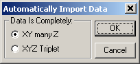
Select the XY many Z format and click OK.

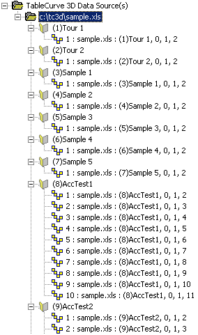
All of the XYZ sets contained within the XLS file have been specified in a single step. All appear as native or intrinsic data items which are displayed in the main graph window using the current 3D graph settings in the Data Graph option.

Select the XYZ data node labeled 1 : sample.xls : (2)Tour 2, 0, 1, 2.

Right click this XYZ item and select Titles from the popup menu.

Default XYZ Titles

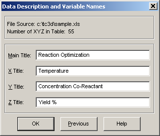
Enter Reaction Optimization for the main title.

We will accept the column titles in the spreadsheet for the X,Y, and Z variables.

Press OK to confirm these titles.

Note that the data item's title in the notebook changes to reflect the revised main title of the data set. This title can also be edited in place directly by clicking on the item after it is already highlighted or via the Rename Selected Item in the right click popup menu.

These are the default titles for this particular XYZ data item. These titles are used throughout TableCurve 3D's various procedures. These titles are stored within the TableCurve 3D Explorer with the data item with which they are associated.

These default titles can be subsequently changed at anytime using the Table menu’s New Titles option, the button in the main toolbar, or by right clicking the specific data item and selecting Titles from the popup menu.

Note that the graphs incorporate these titles only as defaults. A more extensive custom titles option is available in the program’s 3D graphs.

Main Window Graph and Statistics

Non-Parametric Surface Graph

The upper right pane contains the main window graph, a non-parametric surface rendering of the data. The main graph's display will depend on the object currently selected in the TableCurve 3D Explorer. For a native data item, an interpolated surface is rendered. The TableCurve 3D procedure associated with the object is opened by clicking the graph.

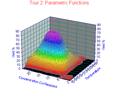
This is a classic two-variable reaction optimization problem where there is an optimum temperature (the X variable in this set) and an optimum level of co-reactant (the Y variable in this set). The purpose of such a DOE (design of experiments) matrix is to find the reaction conditions which result in an optimum yield for the process.

Animating the Main Window Graph

Here we have an excellent example of a surface whose visualization benefits greatly from animation. Note that the 3D peak appears reasonably symmetric at the default viewing angles.

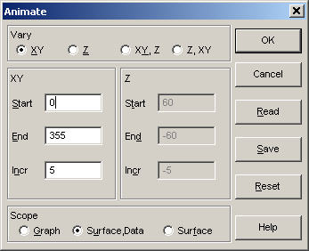
** Select the View menu's Animation Setup item or the equivalent button in the Process toolbar.

**

Be sure the current settings specify XY rotation, starting at 0 degrees and continuing to 355 degrees at an increment of 5 degrees, and a scope of animation consisting of the Surface,Data. Click OK.

The animation is toggled on and off using the Animation item in the View menu or the far right button in the Process toolbar. The animation can remain on while changing items in the notebook.

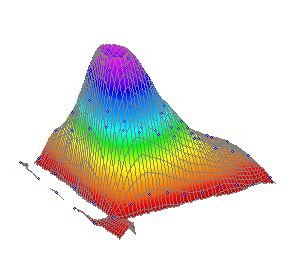
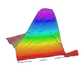
The animation makes it readily clear that the 3D profile is asymmetric in both the temperature and concentration dimensions. A symmetric 3D peak model would have little value for this data.

Select a number of the data set items shown in the notebook. Feel free to explore the sample sets included in the XLS sample file. The animation can remain on as items in the TableCurve 3D Explorer are changed.

At the conclusion, select the XYZ data node labeled Reaction Optimization.

Click the Animation button to stop the animation.

Statistics Summary

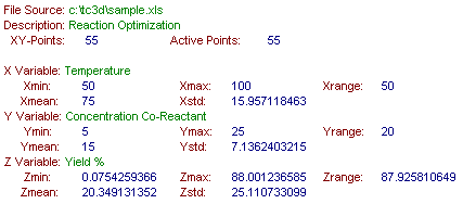
The lower right pane contains the main window statistics, a summary that is specific to the type of object selected. For intrinsic data nodes, this pane will display the basic X, Y, and Z statistics of the data table.

3D Peak Functions

In a multiplicative 3D peak function, the peak is based upon an interaction of both the X and Y variables. In this case, a certain temperature and a certain level of co-reactant are needed to produce a significant yield. At the lower limit of temperature, there is no yield at any co-reactant level. Similarly, at a zero co-reactant level, there is no yield at any temperature.

To understand what TableCurve 3D means by peak type and peak profile, select the View menu’s Non-Linear Sampler option. Chose any peak type and then click the Standard profile and then on the Additive profile.

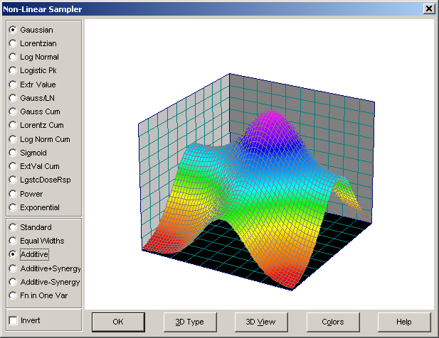
This option very clearly illustrates the difference between a standard (or multiplicative) peak and an additive peak.

Press OK when finished.

Parameters for a Simple 3D Multiplicative Peak

The simplest 3D multiplicative peak contains five parameters:

• An amplitude
• A center value for the X-component of the peak
• A center value for the Y-component of the peak
• A width value for the X-component of the peak
• A width value for the Y-component of the peak

Because a multiplicative peak consists of an X-component peak multiplied by a Y-component peak, only a single amplitude is needed which could represent either peak, the other simply having an amplitude of 1.0.

For the purpose of this tutorial, we will assume that the aim of this surface-fitting is to determine the temperature and co-reactant levels necessary for maximizing yield. Therefore, the two center values are the parameters that are the object of the fit.

Customizing the Surface-Fit

The Surface-Fit Peak Functions in the Process Menu fits all 72 of TableCurve 3D’s built-in non-linear peak functions. For this tutorial, we will save time by fitting only the standard peak functions, those that are likely to match the profile of the data. While a linear model might be able to fit this data, it would be an approximating function only, without coefficients related to the two key center values of interest.

Custom Equation Set

TableCurve 3D offers the means to select the linear and non-linear equations to be fitted.

Select the Process menu’s Edit Custom Equation Set option. Press Clear All in the Linear Equations section and then configure the non-linear equations by checking all six peak types, the Standard profile, and both the None and Add intercept options. The active non-linear equation count should be 14.

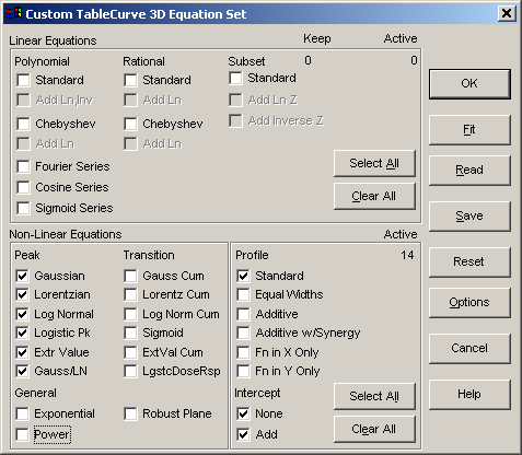
Click OK to close the dialog.

Surface Fit Preferences

Select the Process menu’s Surface-Fit Preferences. Select the F-statistic option in the upper right of the dialog.

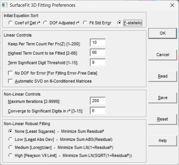
Click OK to close the dialog.

F-statistic

For parametric functions, it is generally best to use the F-statistic sort method which orders the equations based upon how accurately a given model can be said to describe the data. When the equation list is ordered by F-statistic, the simpler but effective equations, those with few coefficients, migrate up the list, while those with many coefficients, however effective, tend to shift to lower positions in the list. In other words, the F-statistic rewards models that are effective in describing the data with few parameters and penalizes models that require a high number of coefficients to do so.

Non-Linear Controls

Non-linear fitting is iterative. Therefore, the maximum number of iterations permitted, as well as the convergence criteria, are selectable. The default iteration maximum of 100 should be sufficient for all except complex UDFs with poor starting estimates. The default convergence precision value of 6 means that the r² must be unchanging in the sixth significant figure for 5 consecutive iterations to signal convergence.

Automated Fitting

Surface-Fit Processing

Select the Surface-Fit Custom Equation Set to begin the fitting. The fit is virtually immediate. Press the Graph Start button at the conclusion of fit.

These 14 equations are fitted quite rapidly. When the fit is complete, these 14 equations will be added to the Review equation list. Successfully fitted non-linear equations are always added to the Review list.

If there is no response to the conclusion of the fit in 10 seconds, the Review is automatically started.

An alternative consists of clicking OK and then selecting the Graph Start item in the Review menu.

Surface-Fit Review

Reviewing the Built-in Peak Model Fits

Click the button for the simplest of the automatic tiling options. The Surface-Fit Graph and Equation List are automatically opened and positioned.

The surface-fit graph for the highest ranked equation is initially displayed:

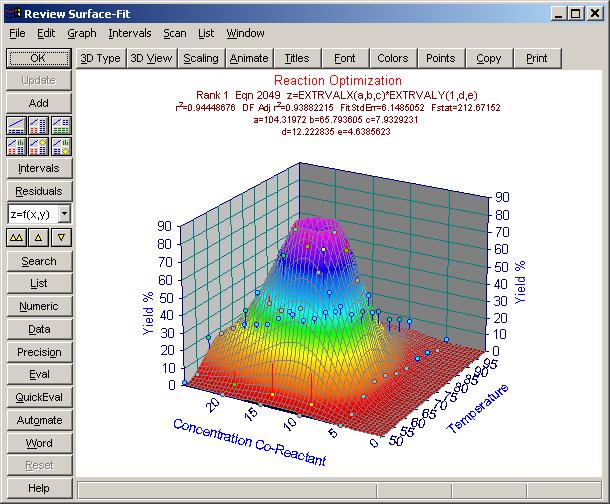
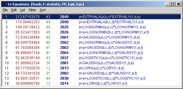
Note that the goodness of fit sort criterion for the equation list is the F-statistic, as displayed in the title bar:

**

Extreme-Value and Log-Normal Peaks

Given the asymmetric nature of the data in both the X and Y dimension, it is not surprising that the Extreme Value and Log-Normal Equations fared better than the symmetric peak functions. The higher the F-statistic, the more accurately a given model can be said to parametrically represent the data.

Note that the addition of an intercept reduces rather than increases the F-statistic for both the Extreme Value and Log Normal multiplicative peaks. This suggests that this data set can be treated as having a zero-baseline since the intercept term is unable to make a significant contribution to the models. Note, however, that the r² is slightly higher for the intercept equations. Here though, we apply our judgment since we know that a zero baseline makes perfect sense for this data set.

Appropriateness of the Model

When there is certainty of an underlying theoretical model, life is often simpler, since there is only one equation to be considered. In this case, we are looking only for a parametric model that accurately describes the maximum yield.

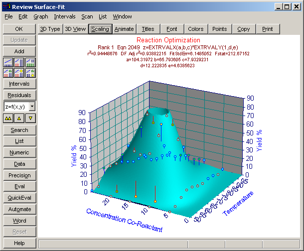
There are a number of factors to be considered. This highest ranked equation has an r² of only 0.944. In this case, we know that this value should be higher since the X and Y values are known to be measured accurately and the Z, the yield, is accurate to within a few percent.

There are other indications that neither the Extreme Value nor the Log-Normal multiplicative peak is fully appropriate to this data set. The manner in which the model fails to adequately cover the anticipated maximum yield of 100% is an important sign that a better model is needed.

Shaded Surface Plot

This type of surface is more easily visualized using a shaded surface plot.

Click 3D Type. Select the type 160 Cyan in the Shaded Plots. Click OK.

Click 3D View. Click Reset. Right click the Mesh Count box and select 120. Click OK.

Adjusting the Graph Scaling

TableCurve 3D's rendering engine truncates the surface at the upper Z scaling limit of 90. Since this optimization is searching for the peak, we will rescale the plot so that the Z upper limit is 100, the theoretical maximum yield.

Select the Scaling item or click in either the left or right Z-axis label area of the surface fit graph. For the Z-axis, click Auto to open the manual scaling and specify 100 as the maximum and 10 for the division count. Press OK and note that this model predicts a maximum yield greater than 100%.

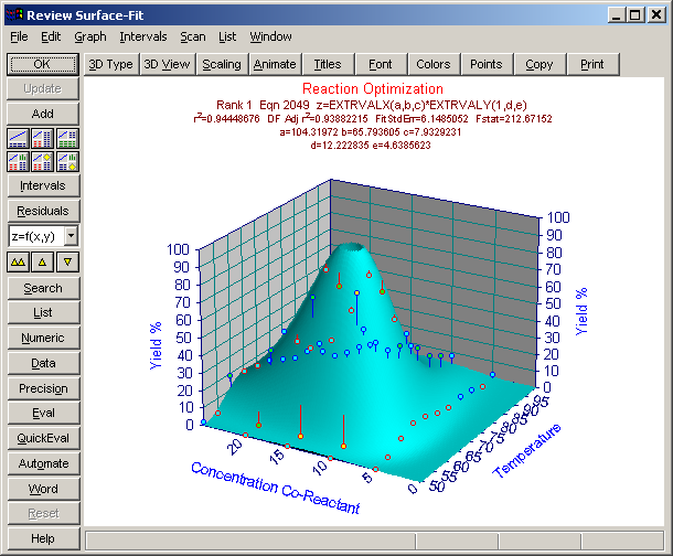
Select the third ranked Log-Normal multiplicative peak. Notice that this model does accurately manage the expected maximum.

Residuals

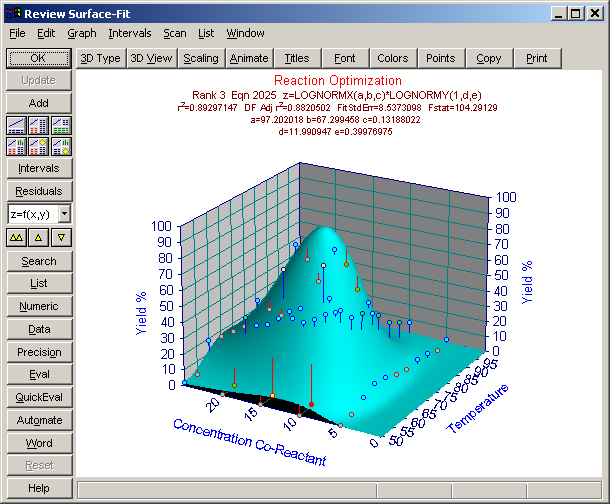
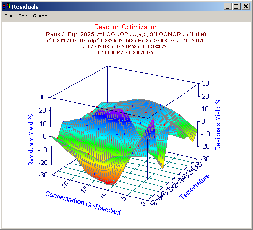
Systematic trends in the residuals are the biggest giveaway to an inappropriate or incomplete model. In three dimensions, the task becomes one of trying to discern whether such trends exist in either the X or Y dimension. Ideally, the residuals surface should be completely random.

With the third-ranked Log-Normal standard peak selected, press the Residuals button. Be sure the Residuals Surface Graph is checked at the bottom of the Graph menu. Note the clear systematic trend in the Temperature dimension.

Check the Residuals Graph in the Graph menu. Select the Point Format option in the Graph menu. Set the size to 5. Click OK.

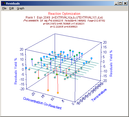
Note that the traditional 3D scatterplot contains a grid drawn at Z=0 and that it is generally easier to see the magnitude and position of the errors. On the other hand, a surface graph is typically better for discerning systematic trends.

When the 4 color option is used for the points, the color fill is based on the number of standard errors from the curve. By default, points less than 1 SE are cyan, those between 1-2 SE are green, those between 2-3 SE are yellow, and those beyond 3 SE are red.

Again check the Residuals Surface Graph in the Graph menu and close the Residuals window.

Random residuals are those that show a high number of sign changes in each direction. In other words, in any given region of the graph there should be a large number of sign changes in the residuals as they are scanned in both dimensions. Note that the strong presence of a systematic trend in one dimension can make it difficult to determine if such a trend exists in the other dimension.

Here the residuals show a clear systematic trend in the X or temperature dimension. What is needed is a peak component in the X dimension that rises far more sharply than either the Extreme Value or Log-Normal peak type.

View Angles

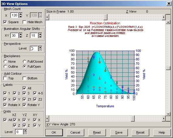
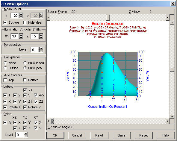
Another way to perceive what is needed is to adjust the view angles to see whether the Log-Normal model is appropriate to the X and Y dimensions. XY view angles of 270° and 0° display the individual profiles. It is a matter of preference whether to zero the Z view angle.

Press the 3D View button or click in the center of the surface fit graph. First set a 270° XY view angle, a 0° Z view angle, and a perspective of 0. Note the clear need for an X peak component with a very sharp rise and very slow decay.

Then set a 0° X-Y view angle. Note that there is nothing to indicate the Log-Normal component is inappropriate to the Y dimension.

Press Reset to restore the default view angles and then OK to return to the surface-fit graph. Click OK to close the Review and return to main window.

User-Defined Functions

At this stage, we can be certain the X component of the model needs a peak that rises very rapidly and decays slowly. Since TableCurve 3D’s most asymmetric peak type is the extreme value, it is necessary to construct a user-defined function to better fit the data. To accomplish this we use the impulse peak model:

4*A0*(1-EXP(-(X-A1)/A2))*EXP(-(X-A1)/A2))

This impulse peak model has a very sharp rise and a slow decay, indicative of the type of profile needed in the X-dimension.

Impulse Peak in X, Extreme Value in Y

The impulse peak function is not available within TableCurve 3D’s built-in functions. We will therefore construct it as a user-defined function (UDF). We will create two user defined functions, both with this impulse function in the X dimension. One uses the Extreme Value function in the Y dimension and the other uses the Log-Normal function.

Select the Process menu’s User Functions item.

TableCurve 3D’s UDF entry screen appears. All 15 of TableCurve 3D’s UDFs are available from this dialog.

Click the Read UDF Library button and then select the UDF library file samplemt.udl. Two user functions will be read and validated. Click OK to acknowledge.

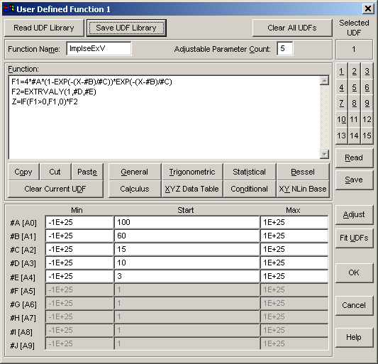
This user function uses the #A, #B, #C, etc. format for the adjustable parameters. The F1 expression is a function for the X-dimension component peak. The F2 expression is a function that uses a built-in non-linear base function, the extreme value peak with Y as the variable. Functions in UDFs are expressions containing X, Y, or an adjustable parameter. Functions must be numbered from F1 through F9. Assignments to any other symbolic names are assumed to be constants. The final Z= expression produces the multiplicative peak function using the conditional IF() function to prevent negative values in the impulse peak.

Graphical Adjustment

Press the Adjust button to open the graphical adjustment dialog. Rather than manually refine the estimates, click Find and Update.

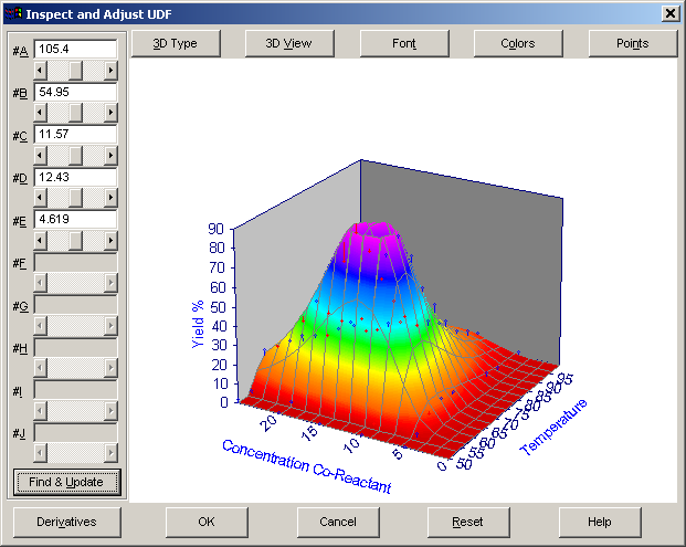
Press OK after the estimates have been updated. Note that the UDF’s estimates in the main UDF screen have also been updated.

The Find and Update option performs a fast reduced point count and reduced tolerance non-linear fit and automatically updates the adjustable parameter fields with the computed estimates.

This graphical adjustment option is extremely important when fitting user-defined functions. When estimates are first refined graphically, the chances of converging to the global minimum, the true least-squares solution, improves considerably.

Adjusting Estimates

When adjusting individual estimates, actual values can be entered or adjustments can be made with the individual scrollbars. The increments in the scroll-bar adjustments will vary with the different parameters and also with the specific value of the parameter. Partial derivatives are computed with each change in a parameter value, and the range of partial derivative across the X and Y data range is used to set the increment for the adjustment. If one or more of the estimates is very far off, the partial derivatives may be so small that the automatic increments will be very large. In such a case, the estimates must be entered manually.

Note that the modified parameter estimates were not saved to the UDF library on disk. To update the UDL file, the Save UDF Library button could have been used.

The Read and Save options save and import a single user function into the UDF position currently active.

We will now adjust the second UDF. Here the Y peak component is based upon the Log-Normal rather than Extreme-Value peak.

Click the 2 button to select the second UDF.

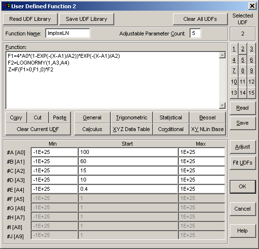
This second user-defined function uses the A0, A1, A2, etc. format for the adjustable parameters rather than #A, #B, #C, etc. Either nomenclature is acceptable. The only other difference between this UDF and the one installed in UDF#1 is that the F2 expression uses a built-in non-linear base function for the Log-Normal function.

Constraints

As with the first UDF, no minimum or maximum constraints are specified. The non-linear least-squares algorithm seeks to produce estimates within specified constraints. If the final parameter values are at a constraint boundary, a true least-squares solution cannot be assumed.

As with the first UDF, press the Adjust button to open the graphical adjustment dialog and again click Find and Update. Press OK after the estimates have been updated. With these refined estimates in the main UDF entry screen, press OK to return to the main menu.

Fitting Only the UDFs

There is a Fit UDFs button in the main UDF screen and a Process menu Surface-Fit User Functions option. Both initiate the fitting of only the UDFs. There is no limit on the single UDFs or UDL libraries saved to disk, although only fifteen UDFs may be included in the surface-fitting at any given time.

For this tutorial, we want to have the Extreme Value and Log-Normal standard peaks that were previously fitted available as a reference for readily determining if these UDFs with the impulse peak offer significant improvement. We will thus modify the custom set to include only these two peak types. All fit options, including the Surface-Fit Custom Equation Set option, automatically include installed UDFs.

Select the Process menu’s Edit Custom Equation Set option. Press Clear All in the Non-Linear Equations section and then check only the Log-Normal and Extr Value peak types. The active non-linear equation count should be 2. Click the Fit button.

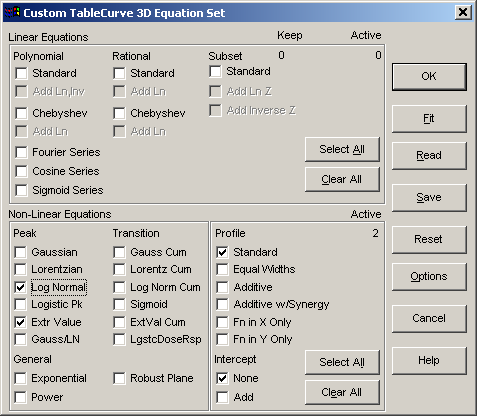
The fit should proceed rapidly with the two built-in non-linear equations being fitted followed by the two UDFs. Four total equations will be added to the Review equation list.

Select the Graph Start option to begin the Review.

Graphical Surface-Fit Review of User Functions

Impulse-Log Normal Fit

Scaling is not preserved when leaving the Review. Since we did not save the 100% Yield scaling to file, we must re-enter the scaling.

Select the Scaling item or click in either the left or right Z-axis label area of the surface fit graph. For the Z-axis, click Auto to open the manual scaling and specify 100 as the maximum and 10 for the division count. Press OK and note that this model predicts a maximum yield very close to 100%.

Since the surafce rises so sharply, we will create a photorealistic surface to improve visualization. This is achieved by specifying a very high mesh count for a shaded surface plot.

Click 3D View, right click the Mesh Count edit field and select 240 for the mesh count. Click OK.

With this photorealistic rendering, it is possible to observe that the peak ever so slightly crosses the 100% theoretical maximum yield threshold.

Click Points, select Visible Only, and click OK.

The Visible Points option in the Points dialog offers the means to hide those points associated with the portion of the peak hidden from view. Each point is associated with a surface mesh element. It is that mesh element to which the Z-drop line is drawn.

Note that the Visible Points option has to do with the visibility of the mesh element with which the point is associated, not to the actual visibility of a point itself. If the whole of a surface is visible, this option has no effect, other than to slow the rendering of the graph.

This Visible Only option makes clearer that very few points define the sharp upward rise of the impulse-component of the peak. In general, it is best to use the All Points option. It is faster and there is no danger of missing an outlier because a specific point was associated with a hidden mesh element and not drawn.

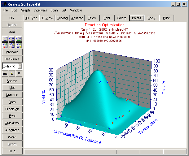
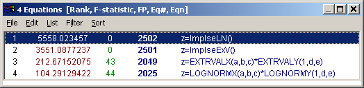
Note the major improvement in F statistic with the UDFs. The X-component impulse peak makes a substantial improvement in the fit. The r² is also 0.997 for this highest ranked Impulse-Log Normal peak.

While the Impulse-Extreme Value peak is also highly ranked, the Impulse-Log Normal produces a better F-statistic, an indication it is a better model for describing the data.

Impulse-Extreme Value Fit

Click the down arrow button in the Surface-Fit graph’s control panel.

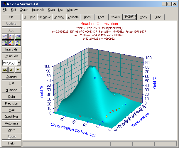
This selects the second ranked Impulse-Extreme Value UDF. Here the peak in the surface exceeds the 100% theoretical maximum in a more obvious manner. This model has an r² of 0.996.

Residuals Graph

Click the Residuals button.

Select 3D Type in the Graph Menu of the Residuals window. Click Reset. Click OK.

Select 3D View in the Graph Menu of the Residuals window. Click Reset. Set a 270° XY view angle, a 90° XY view angle, and a perspective of 0. Set Size in Frame to 0.85. Click OK.

Using either the arrow buttons or by direct selection in the Equation list, view the Residuals for the two UDFs and the two built in peak functions.

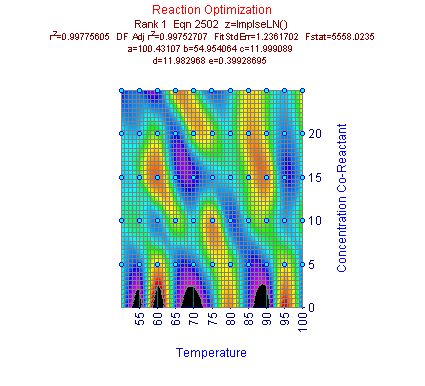
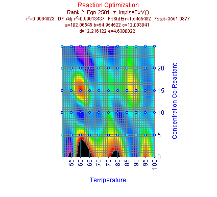
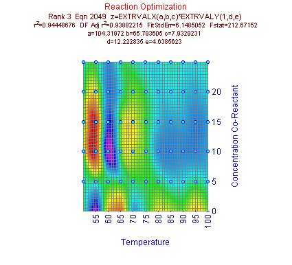
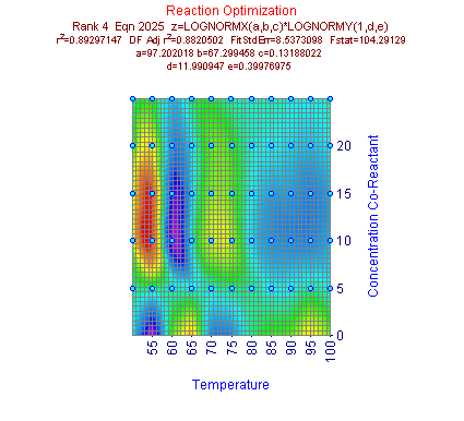
The contour plots make it very clear that the residuals for the built in peak models show substantial systematic trends. The UDF with the extreme value component is better. The UDF with the log normal component produces a fit whose residuals are very close to randomly distributed.

Select 3D View in the Graph Menu of the Residuals window. Click Reset. Click OK. Close the Residuals window.

Prediction Intervals

Select the top ranked ImpulseLN user defined function.

Using the Intervals menu, click 99% as the confidence level and select Prediction Intervals.

Click 3D View. Click Reset. Set a 290° XY view angle. Click OK.

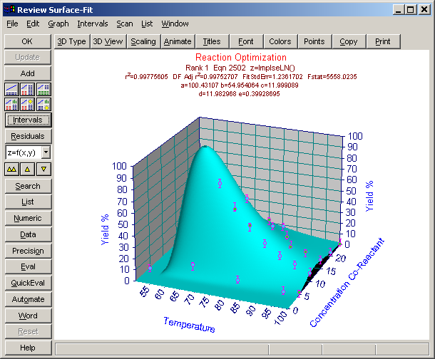
Note that the prediction intervals appear to be reasonably uniform across the domain of the surface.

Animating the Surface-Fit Graph

Click the Animate button and set the animation to Vary XY, and to start at 5°, end at 360°, using 5° increments. Press OK to open the animation window. Click Start to begin the animation. Observe the surface and data at the various angles, and the click Stop to halt the animation and then End to close the animation window.

Click 3D Type. Click Reset, and then OK to reset the default gradient plot.

Click 3D View. Click Reset. Click OK to reset the default view angles.

Click Points. Click Reset. Click OK to restore all point plotting.

Click Intervals to toggle off the drawing of prediction intervals.

Numeric Surface-Fit Review of User Functions

For the remainder of this tutorial we will explore numeric options.

Real Time Evaluation

TableCurve 3D has a feature that is particularly useful when optimizations involve the search for a global minimum or maximum in the surface.

Click QuickEval and check the Surface Max box. Step through or select the four equations and note the X,Y positions of the optimum and the predicted maximum yields for each.

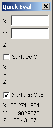
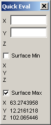
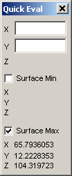
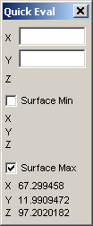
The goal of this tutorial is to optimize the reaction conditions for maximum yield, that is, to find the temperature and co-reactant concentration which maximized product yield. The best fit equation has a surface maximum at 63.3 °C and 12.0 concentration. The second UDF has its maximum at 63.3 °C and 12.2 concentration.

Click QuickEval again to close the quick evaluation window.

Numeric Summary

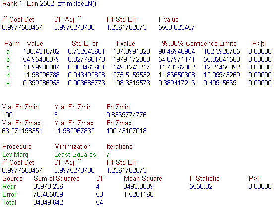
The Numeric Summary provides important statistical information regarding the parameter values, the standard errors for the parameters, the confidence interval about the parameters, and the extrema of the function.

To illustrate the benefits of having separate measured values for the maxima and minima of a UDF, we have deliberately used a parameterization for the impulse peak function that does not directly produce the center value. For the UDFs used, the impulse center value will actually be a1+a2*ln(2).

Select the highest ranked Impulse Log-Normal equation and click the Numeric button. Note the statistics of fit for this highest ranked UDF.

When finished, close the Numeric Summary window.

Optimization Analysis

The Log-Normal center is 11.983, the d-parameter. Note also that the measured value of Y at Fn Zmax is likewise 11.983. Thus the optimum concentration of co-reactant has been determined to be essentially 12.0. The Impulse center is 54.95, the b-parameter, but the measured X at Fn Zmax is 63.27. Clearly the parameterization of the impulse peak does not provide a true Z max center. In this case, we know the center of the peak occurs at b+c*ln(2) which is 63.27, confirming that the optimum temperature is about 63.3°.

For the statistics to have the fullest possible meaning, the impulse peak should be reparametrized so that the b parameter is the true center of the impulse peak. This is left as an optional exercise for additional experience with UDFs. (Hint: replace the A1 parameter in the UDF F1 expression with (A1-A2*LN(2)). If successful, the X at FnZmax will match the b-parameter).

Note that the surface minimum and maximum values reported in the Numeric Summary and in the Quick Eval option use a two-dimensional minimization algorithm which is not immune to local minima. Use these measured values only in conjunction with careful graphical inspection of the surface.

In this example, the largest t-values are for the two center values, suggesting these have been the parameters most strongly determined to be non-zero. This good news results in the excellent 99% confidence intervals about the two location parameters in the model.

Data Summary

Click the Data button and observe that the highest yield data point of Temperature=65, Concentration=10 has an observed yield of 88% and a predicted yield of 89.0%.

When finished, close the Data window.

Given that this data set consists of the observations of 55 separate reactions, with only eight above a 50% yield, an experimenter might readily accept the [65,10] conditions with this 88-89% yield to be an optimum. Surface-fitting offers an optimization strictly by analytical means. With only the surface fit analysis, it is possible to project a near complete yield at [63.3,12].

Of course, no self-respecting scientist relies entirely upon such an analytical approach. If resources permitted, the ideal situation would be another design of experiments matrix covering a much narrower range of temperatures and concentrations, these being centered about [63.3,12].

Evaluation

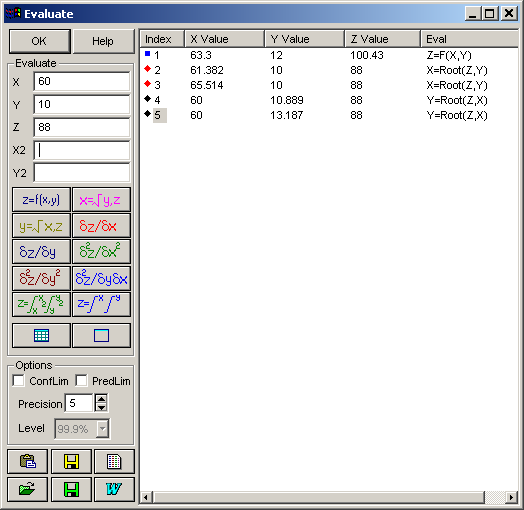
To confirm this near-ideal yield at [63.3,12], click Eval and then enter 63.3 as the X value and 12 as the Y value. Click Z=F(X,Y) and note that a yield of 100.4% is calculated.

To check the model near the maximum yield actually observed in the experiment, enter 60 as the X value and 88 as the Z value and then click Root at Z,X. The root-finder reports two roots, one at a concentration of 11 and one at 13, the first being close to the experimental concentration of 10.

Next enter 10 for the Y value and click Root at Z,Y. The root-finder again reports two roots, one at a temperature of 61.4 and one at 65.5, the latter being close to the experimental temperature of 65.

Partial Extrapolation

It is worth noting that while the [63.3,12] is well within the X and Y range of the data, its predicted Z is one which does not exist anywhere within the data set. It is possible that a limiting factor may be present only above 90 or 95% yield, and the dynamics of such a process will not be manifested anywhere within the data in this experiment. While this is not a full extrapolation, it is nonetheless a partial one since the sampled Z range does not include the predicted Z of the optimum. This is a fundamental issue for all maximum or minimum type optimizations. Therefore, experimental confirmation of the estimated optimum is essential.

Click OK (or click again on the Eval button, if visible) to close the Evaluation.

Click Add to add this surface fit to the TableCurve 3D notebook.

Click OK in the Surface-Fit graph to exit the Review and return to the main program window.

Surface Fit Output Items

TableCurve 3D stores the necessary information to recreate all of the fits available in the Review, but does not save the results of all of the fits. When the main window graph is clicked, and it reflects a surface fit, the equations previously fitted are again fitted using the same preferences previously applied.

Select the first of the six surface fit items and click in the center the main graph window.

This places the Review in the state it was in when this surface fit item was previously added to the TableCurve 3D notebook. The same equations are available in the Equation List and the equation comprising the surface fit object will be selected. Any graph customizations previously made are also restored.

Click the OK button in the Surface-Fit graph to once again exit the Review and return to the main program window.

Annotation Items

These items are useful for adding experimental notes to a TableCurve 3D notebook file. An annotation item can only be added to an XYZ data node.

Select (left-click) an XYZ data item in the notebook hierarchy and then right click the item to open the popup menu. Select Annotate. Enter a few words or lines into the editor that overlays the statistics window. Close the Annotation window.

When an annotation item is selected, its text is displayed in the statistics window. Since the ASCII editor can open any ASCII file, the content of such files can be easily added to the TableCurve 3D notebook file.

Exiting TableCurve 3D

To exit TableCurve 3D, either close the main TableCurve 3D window, or use the Exit item in the main File menu.

The first tutorial covers approximating functions and focuses on TableCurve 3D’s linear equations and general operations.