Edit Custom Equation Set
The Edit Custom Equation Set option in the Process menu is used to configure a custom equation set for TableCurve 3D's automated fitting. Here you select linear families of equations or specific types of non-linear equations to be included in the equation set that is fitted.
 The equation selections apply only to the Surface-Fit Custom Equation Set fitting option. You may save a custom equation set to disk for recall at any future time.
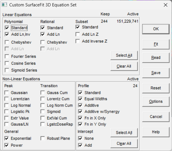
Linear Equations
The Standard XY polynomials consist of 27 polynomials based upon X and Y. These include two Taylor polynomials which contain at least one X-Y interaction term. The Add Ln,Inv item expands the polynomials to 243 total equations based upon X, ln(X), 1/X, Y, ln(Y), and 1/Y. These consist of 225 non-interactive equations, and 18 Taylor polynomials which include X-Y interaction terms.
The Chebyshev polynomials add 9 polynomials through true tenth order bivariate. The Add Ln item adds 27 additional equations that include ln(X) and/or ln(Y). The Fourier Series option adds 9 simple and 4 bivariate models. The Cosine Series item adds 9 models as does the Sigmoid Series option.
The Standard XY rationals consist of 65 rationals based upon X and Y, one of which consists of a Taylor series numerator and denominator. The Add Ln item expands the rationals to 260 total equations based upon X, ln(X), Y. and ln(Y), 4 of which contain Taylor series numerators and denominators. Note that all rational equations, by their very nature, model X-Y interactions.
The Chebyshev rationals add 10 models through 10/11 order. The Add Ln option adds 30 models that include ln(X) and/or ln(Y).
The Standard Selective Subset will fit up to 12,194 equations without a Z-transform, selecting from 151,232,238 total equations. The Add Ln Z item adds up to another 12,194 equations based upon a ln(Z) transform, these equations also selected from 151,232,238 equations. The Add Inverse Z is similar except that a 1/Z transform is used. When all subset items are checked, up to 36,582 equations will be fitted from a total set of 453,696,714. Note that the Z-transform subset fits will be terminated early if the best of the 3-coefficient fits is poorer than the worst of the standard 3 coefficient subset fits added to the equation list.
You may click on Clear All to clear all linear equations and on Select All to activate all linear equations. The TableCurve 3D equations are listed in the appendix of the manual and can be viewed by using the Equation List Help items in the main menu's Help.
Non-Linear Equations
In TableCurve 3D you must select an equation type and an equation profile. To see what is meant by the various 3D profiles available, you should explore the various profiles in the View menu's Non-Linear Sampler option.
It takes a considerable time for TableCurve 3D to fit all non-linear equations, and as such, selecting only the profiles of interest can significantly reduce fitting time.
You must also choose either to fit without a Z-intercept(None), with a Z-intercept(Add), or to do both type of fits.
You may click on Clear All to clear all non-linear equations and on Select All to activate all non-linear equations.
The 168 built-in non-linear equations can be viewed in both a full and notational format in the Help menu’s Non-Linear List option:
The notational format is used in the titles of the TableCurve 3D surface-fit and residuals graphs. The notational format enables an immediate recognition of the profile. For example, the Gaussian-based non-linear functions use the following notation:
2001 z=GAUSSX(a,b,c)*GAUSSY(1,d,e)
2002 z=a+GAUSSX(b,c,d)*GAUSSY(1,e,f)
This is the Standard profile with and without an intercept. Note that the Gaussian in X is multiplied by the Gaussian in Y. The standard or multiplicative profile often relates to dynamic situations where Z depends entirely upon the interaction of X and Y. For example, X may be the concentration of one reactant, Y the concentration of another reactant, and Z the overall yield or some other measured parameter. In the Standard equations there is a distinct width parameter for both the X and Y dimensions.
2003 z=GAUSSX(a,b,c)*GAUSSY(1,d,c)
2004 z=a+GAUSSX(b,c,d)*GAUSSY(1,e,d)
These Equal Width profile equations are identical to the Standard equations except that both Gaussian components now share a single width. This produces a purely symmetric peak. Viewed from a 0° Z View Angle, such a peak would have a constant width regardless of XY View Angle.
2005 z=GAUSSX(a,b,c)+GAUSSY(d,e,f)
2006 z=a+GAUSSX(b,c,d)+GAUSSY(e,f,g)
These are the Additive profile Gaussian equations with and without an intercept. Note that the Gaussian in X is added to the Gaussian in Y. The additive profile often relates to situations where Z varies with X and Y in an independent fashion. For example, X may be the concentration of a catalyst, Y the concentration of an independent co-catalyst, and Z the overall yield or some other measured parameter. In the Additive equations there is a distinct width parameter for both the X and Y dimensions.
2011 z=GAUSSX(a,b,c)+GAUSSY(d,e,f)+GAUSSX(g,b,c)*GAUSSY(1,e,f)
2012 z=a+GAUSSX(b,c,d)+GAUSSY(e,f,g)+GAUSSX(h,c,d)*GAUSSY(1,f,g)
These are the Additive w/Synergy profile Gaussian equations with and without an intercept. Here there is a sum of the Additive and Standard profiles. The additive w/synergy profile relates to situations where Z varies with X and Y in both an independent and interactive fashion. For example, X may be the concentration of a catalyst, Y the concentration of a second catalyst whose activity is either increase d or decreased by the presence of the first catalyst, and Z the overall yield or some other measured parameter. In the Additive w/Synergy equations there is a distinct width parameter for both the X and Y dimensions and a separate magnitude for the additive and multiplicative components.
2007 z=a+by+GAUSSX(c,d,e)
2008 z=a+bx+GAUSSY(c,d,e)
2009 z=a+by+cy2
2010 z=a+bx+cx2
These are the Fn in X Only and Fn in Y Only profile Gaussian equations. The first two equations offer a linear fit in the non-Gaussian dimension and the second two offer a quadratic fit. These equations are of use when Z depends on only one variable in a non-linear fashion and where the other variable can be fitted linearly with a basic function. For example, X may be the concentration of a catalyst, Y the temperature, and Z the overall yield or some other measured parameter. The catalytic impact on Z might be Gaussian while the temperature impact is parabolic and fitted by a simple quadratic.
All of TableCurve 3D’s built-in non-linear equations follow this same basic structure except the Gaussian/LN option. Because it is very common in nature and in statistical procedures to have a three dimensional distribution that is Gaussian in one-dimension and Log-Normal in the other, TableCurve 3D includes this special case of mixed functions. For this special mixed function, the Equal Widths and Fn in X Only, and Fn in Y only profiles have no meaning. There are four Standard functions, four Additive functions, and four Additive w/Synergy functions.
It would be impossible to include all possible combinations of even the built-in non-linear base functions. For example, you might have data that has a peak profile in one dimension and a transition profile in another. You might have a transition function that is clearly symmetric in one dimension but quite asymmetric in the other.
The purpose of TableCurve 3D’s notational format is not only to present a complex equation in the simplest possible way, but also to enable easy construction of User-Defined Functions. TableCurve 3D’s built-in non-linear base functions use this notational format and can be based upon X, Y, or $, the variable of integration. By using these built-in non-linear base functions you can readily construct a specific UDF. For example, for data with a very sharp right asymmetric peak shape in the X dimension and an exponential decay in the Y dimension, the following UDF might be appropriate:
F1=EXTRVALX(A1,A2,A3)
Fit Controls
Linear and non-linear fitting controls for fitting this custom equation set are configured in the Process menu's Surface-Fit Preferences option. To set these controls from this custom equation set dialog, simply click the Options button.
Saving a Custom Equation Set
Use the Save item to save the current equation set to disk. The default file extension is FIT. These are binary files that can only be produced within the program. Custom fit files can be recalled at anytime. The current custom fit is always saved across sessions. You will want to save custom fits to disk if you plan to use more than one custom set in your work.
Reading a Custom Equation Set
Use the Read item to read a custom equation set from disk. The current settings will be updated to reflect this new configuration. You may also use the Read Custom Equation Set Process menu option to read a custom fit configuration.
Reset
Use the Reset button to restore the configuration present when the dialog was opened.
Fitting a Custom Fit Configuration
Use the Fit item to immediately fit the equation set shown. This is the same as using the Surface-Fit Custom Equation Set option in the Process menu.