Questions and Answers¶

Automated Fitting¶

Where do I start?

TableCurve 3D has been designed to automatically fit large numbers of candidate surface-fit equations in a fully automated fashion. In general, there are four basic steps.

1. Set up an an XYZ Data Table¶

Use the Import Data Source option to add a disk-based file containing one or more XYZ data sets to the current notebook. This option is available from the main File menu, in the main toolbar, and when right clicking the uppermost or notebook item in the TableCurve 3D Explorer.

Supported formats include ASCII, Excel, Lotus 123, Quattro Pro, SigmaPlot, SPSS, Systat, DIF, and dBase.

XYZ data sets are subsequently specified using a variety of approaches:

The Autospecify All XYZ Data Items option is the easiest way to specify all XYZ data sets in the entirety of a data source, such as an Excel file. This option is in the File menu and in the right click menu for the data source item, or if expanded, for the individual sheets within a spreadsheet file.
The Specify XYZ Data Item option is used to specify the X, Y, and Z columns for a single data set. This option is also in the File menu and in the right click menu for the individual sheets within a spreadsheet file.
If the data source is a three column ASCII file or an SPSS file exported from TableCurve 3D, the XYZ variables and the titles are automatically specified.

Use the TableCurve 3D Editor option in the Edit menu to manually enter XYZ data for use within TableCurve 3D.

2. Process the Data for the Best Equations¶

The following fitting options in the Process menu or process toolbar utilize pre-defined equation sets:

3. Select the Optimum Equation for the Application¶

TableCurve 3D offers a large number of graphical and numerical tools to enable you to choose the best equation for your particular needs.

For selecting the most appropriate equation, the Review menu’s Graph Start option emphasizes the Surface-Fit Graph.
The Review menu’s List Start option emphasizes the Equation List.

4. Generate the Printed, File, or Code Output¶

The Save Excel, Save SigmaPlot Win, and Save ASCII items in the Review Surface-Fit Graph’s File menu are the most commonly used file export options.

The Print option in the Surface-Fit or Residuals Graph is used to generate printed graphs. The Copy option can be used to create disk or clipboard-based bitmaps or metafiles.

Statistical reports can be printed, copied to the clipboard, streamed to MS Word, or saved as RTF (rich-text format) files.

The Code Generation option, in the Surface-Fit Graph’s File menu, is used to generate the fitted equation in C, FORTRAN 77 or 90, Pascal, BASIC, C++, Matlab or Java.

Data Table I/O¶

How do I import data from external files?

Add the data source to the TableCurve 3D notebook using the Import Data Source option. This option is available from the main File menu, in the main toolbar, and when right clicking the uppermost or notebook item in the TableCurve 3D Explorer.

Specify the XYZ data set(s):

The Autospecify All XYZ Data Items option specifies all XYZ data sets in the entirety of a data source, such as an Excel file. This option is in the File menu and in the right click menu for the data source item, or if expanded, for the individual sheets within a spreadsheet file.
The Specify XYZ Data Item option is used to specify the X, Y, and Z columns for a single data set. This option is also in the File menu and in the right click menu for the individual sheets within a spreadsheet file.
If the data source is a three column ASCII file or an SPSS file exported from TableCurve 3D, the XYZ variables and the titles are automatically specified.

For an individual XYZ specification. you may optionally specify a weights column or a column containing the standard deviation of replicate measurements.

How do I paste in the data from the clipboard?

Use the Import Clipboard option included in the Import Special menu list in the File menu. This option is also available in the main toolbar.

The clipboard block can contain any number of columns. To make it possible to paste many XYZ sets from a single clipboard operation, TableCurve 3D first saves the contents of the clipboard to a disk file. This file is automatically added to the TableCurve 3D explorer as a data source.

The XYZ data sets are then specified using the The Autospecify All XYZ Data Items option or the Specify XYZ Data Item option.

My data are in a spreadsheet with the X values in the first column, the Y values in the first row, and the Z values in the matrix defined by the X and Y values. How do I import this format?

This type of matrix cannot be imported directly from a file. Copy the spreadsheet matrix to the clipboard and use the Import Clipboard Matrix option included in the Import Special menu list in the File menu. The cell in the first copied row and column should be empty. The data is saved to disk and added as a WK1 or WK3 data source to the TableCurve 3D explorer.

How do I append data to the existing data table?

Using the TableCurve 3D explorer, drag one of the data sets onto the other. The order does not matter. An Appended Data folder is created and a new XYZ data item is created in this folder. The new data item represents the result of appending the two sets.

How does the File menu’s digital filter work?

The Digital Filter option is one of the import options included in the Import Special menu list in the File menu. The Set Digital Filter and Apply Digital Filter options are also available in the right click popup menu of non data and data nodes in the TableCurve 3D Explorer.

Beginning at a specified starting position, every nth data point in the incoming data stream is added to the XYZ data table. This approach should only be used for very large data sets where the loss of data observations can be tolerated. Generally, this option is used for importing data tables greater than the program’s 16384 data point limit.

What is the best overall approach for digitally reducing or enhancing data?

The Non-Parametric menu’s Interpolate to Uniform Grid option can be used to digitally reduce or enhance data. The output grid is uniform and the number of x and y points in the grid can be independently set.

How do I drag and drop data sources into TableCurve 3D?

Simply drag the file(s) from Windows Explorer into the main TableCurve 3D window.

How do I save the data table in an alternative format?

In addition to the default ASCII format, the Export XYZ option in the File menu offers Excel, WK3, WK1, Systat, and SPSS binary data formats.

How do I copy the data table to the clipboard?

Use the Edit menu’s Copy Current XYZ Data option. The clipboard contains both ASCII and spreadsheet binary data formats.

Data Input¶

How do I input data while simultaneously graphing it?

Use the TableCurve 3D Editor option in the Edit menu and activate the Graph button after 4 or more points have been entered.

How do I reverse or swap variables?

This can be done in the TableCurve 3D Editor using the Reverse button.

Although TableCurve 3D sorts the data primarily by ascending X, and secondarily by ascending Y, can I save the data unsorted or in some other sort order?

Yes. You must save the data while you are within the TableCurve 3D Editor since the data table is automatically sorted when you return to the main menu. The editor also contains a Sort Table option which offers ten different sorts.

My X and/or Y values are equally spaced. Do I need to enter each of these in the TableCurve 3D Editor?

No. Turn on the AutoEntry X and/or AutoEntry Y. After two values have been entered, all subsequent entries will be automatic.

Can I have a transformation applied after entering values?

Yes. Use the Calculation option in the TableCurve 3D Editor to enter the transform. Be sure Apply New is checked.

Can I enter or edit the data table using a simple ASCII editor?

Use the ASCII Editor option in the Edit menu.

What is the best way to assign weights to data?

Weighting of fits is used to compensate for a variety of factors. The most common is to weight the data based upon uncertainty. When each point represents the average from multiple observations, weights are generally set to inverse variances (1/SD²). When each point represents a single observation, the weights can represent a measure of experimental uncertainty for that element of the data.

Weighting is sometimes used to compensate for limitations within the least-squares process, especially when the Z values span several orders of magnitude or more. It is often simplest and most effective, however, to apply a Z=LN(Z) calculation prior to fitting rather than using weighting.

Data Preparation¶

How do I transform one or more columns in the data?

Use the Calculate menu’s Enter Calculation option. The X column is treated as a vector with the name X, the Y column with the name Y, the Z column with the name Z, and the weight column with the name W. To convert X values in cm to micrometers, for example, enter X*1E4 in the X= field.

All of TableCurve 3D’s built-in functions are available in a simple push button help where the desired functions are automatically inserted into the expression.

How do I smooth data prior to fitting?

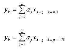Generally, you will use the Smooth Loess option in the Table menu. This option accepts both gridded and scattered data and offers the greatest control of smoothing power.

The Smooth NURBS option offers the intrinsic smoothing of non-uniform rational B-splines and may be of value with gridded data.

Although my data were originally on an X,Y grid, I was forced to disable several points containing artifacts. Is there a way to perform a local interpolation to restore the grid?

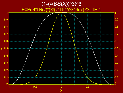The Fill Sparse Grid option in the Non-Parametric menu offers a host of scattered data algorithms that will interpolate missing positions within a grid. The data table is automatically updated.

How do I generate a uniform grid of interpolated values from scattered data?

One approach is to perform a surface fit of all or selected models. After choosing an appropriate equation, the Eval option’s Generate Table procedure can be used to interpolate a uniform grid of the desired density.

A fast alternative is to use the Interpolate to Uniform Grid option in the Non-Parametric menu. This option replaces the current data table with the result of a scattered data interpolation.

What are the advantages and disadvantages of using a non-parametric procedure to generate a uniform interpolated grid prior to fitting?

Large void regions in the XY domain of scattered data often result in a non-constrained condition with parametric fits. Preprocessing to a uniform grid generated by a non-parametric local fitting procedure can furnish the necessary constraints, stabilizing the fits of complex polynomials and rationals. The drawback to this approach is that additional error is introduced by the interpolation step.

What is the best approach for data reduction prior to import and fitting?

If the data stream contains more than the 16,384 entries, you should use the Import Digital Filter option. With this option, some observations are discarded.

In all other cases, the Interpolate to Uniform Grid option should be used because all observations will factor into the interpolation.

How do I remove the current XYZ data?

Remove the XYZ data item in the TableCurve 3D explorer. If the data source contains only a single XYZ set, delete the data source.

How do I clear all items in the current notebook?

Use the New... item in the File menu, the main toolbar, or in the right click popup menu when on the uppermost item in the explorer.

How do I change the basic data table titles of an XYZ data set after import?

Use the New Titles option in the Table menu or the Titles option when right clicking a native XYZ data item. The Rename Selected Item in the File menu and right click popup menu is used to rename the current item in the notebook. This also modifies the default main title for the data set.

How can I graphically turn individual points off so that they will not be used in the fitting?

Use the Section Data option in the View menu to create a Section object. Toggling a point on and off is as simple as left clicking on that point with the mouse. Regions of data can be excluded or included by setting and applying numerical limits.

In some cases, all I need is a printout of the basic data table statistics shown in the statistics window. Can this be done?

Yes. Use the XYZ Statistics option in the Table menu. A full range of print and copy options are available.

What is meant by gridded or scattered data?

Data on a grid consist of a matrix of increasing X and Y values for which an observation exists for each X,Y position. In TableCurve 3D, a uniform grid is not needed for procedures which require gridded data. Scattered data are simply those that are not present on a rectangular grid.

Since the Estimate Gridded Data and Smooth NURBS option require gridded data, why is it possible to process scattered data?

TableCurve 3D automatically uses a scattered data interpolation algorithm (Renka I) in a preprocessing step when a regular grid is absent.

I only need to view one or more smooth partial derivatives of the input data. How can I do this?

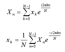
Use the Estimate Gridded Data or Estimate Scattered Data option in the Non-Parametric menu. All five first and second order partial are available for display and evaluation.

The Renka I procedure in the Estimate Scattered Data option is particularly effective in generating smooth and accurate partial derivative surfaces.

Viewing Arbitrary Functions¶

How do I graph an arbitrary function of X and Y?

Use the View menu’s Function(X,Y) option. This option allows a multi-line function of X and Y to be graphed. All of TableCurve 3D’s built-in functions are available in a simple push button help where the desired functions are automatically inserted into the expression.

I need to create a fast approximation for a computationally intense function of X and Y. How do I generate full precision data for subsequent fitting?

You can generate data from the Function(X,Y) option. Use the Eval option from the graph of the function. The Generate Table option can be used to create full 19-digit precision data. The best approach is to write to the evaluation table and then use the Save Data to Disk option. The Lotus WK3 option is recommended for preserving full binary precision.

If you use an external program such as Maple, Macsyma, or Mathematica to produce high-precision ASCII data for TableCurve 3D, set the arbitrary precision to at least 20 digits. All routines requiring a specified convergence should be set to a tolerance of 1E-18 or smaller.

Non-Parametric Estimation¶

With all of TableCurve 3D’s parametric fitting options, why would I want to use a non-parametric procedure?

If your data set has a very unusual profile, it is possible that none of TableCurve 3D’s built-in equations will fully describe the features within the data. In some cases, a non-parametric fit may succeed.

If you need only a few simple interpolations, a non-parametric procedure offers near immediate processing, and the same evaluation procedure as that of the parametric fitting.

I see that the Non-Parametric menu offers both gridded and scattered data estimation. Is there a significant advantage to using fully gridded data?

The better scattered data algorithms, when processing data on a grid, are nearly as accurate as the tensor product splines which offer the best accuracy of the gridded procedures. However, data on a uniform grid represents an optimum condition for interpolation and extrapolation.

Which of the non-parametric procedures offer extrapolation?

The Bicubic+Akima, Akima III, and NURBS options offer extrapolation in the Estimate Gridded Data option.

In the Estimate Scattered Data option, all procedures offer extrapolation.

Why should I choose one algorithm over another?

Each of the non-parametric procedures has its own strengths and limitations. These are discussed at length in the descriptions for each of the procedures.

Surface-Fitting¶

With so many built-in equations, how can I gain an understanding of the various groups or types of equations?

The Equation List Help item in the Help menu offers the following listing of equations:

The Edit Custom Equation Set option also offers the means to customize an equation set from the full set of built-in equations.

How do I decide which equations should be fit?

This is the premise of TableCurve 3D. The product assumes it is not often easy to know which equations may be appropriate to a given data set. Until you gain certain experience with the product, it is a simple matter to fit All Equations to the data.

All other fitting options for built-in equations represent conveniences to save fitting time. Since the Review’s equation list can be filtered and sorted in a number of ways after the fact, it is not necessary to limit the list of candidate equations by restricting the set being fitted.

What is a Chebyshev polynomial or rational equation?

The Chebyshev series is a type of orthogonal polynomial defined from -1.0 to 1.0. TableCurve 3D’s Chebyshev polynomials and rationals consist of a sum of sequential series terms. The X and Y values are scaled so that the X and Y ranges are mapped to this -1 to 1 defined range. Because of the scaling and complexity of the series term evaluation, a separate procedure is needed in the code generation options. A Chebyshev polynomial offers significant advantages in terms of stability. Bivariate polynomials up to 10th order (66 terms) can be fitted without encountering ill-conditioning.

What is a Fourier series equation?

A standard Fourier series consists of independent x and y sine and cosine terms and is essentially a least-squares overdetermined FFT. A bivariate Fourier series contains x,y interaction terms and is generally of greater value in surface fitting. A bivariate cosine series is similar, but contains only cosine terms. These series are also scaled equations, from 0 to p.

What is a Sigmoid series equation?

These are empirical models whose basis functions are scaled sigmoids. These functions can often model sharp transitions which appear within surfaces.

How about a brief overview of Process menu fitting options?

All Equations: fits or selects from all built-in equations. This is the recommended option until you become more familiar with the equations.

Linear Equations: all linear equations; omits the built-in non-linear equations. This is often a good option when searching for an approximating function.

Simple Equations: fits all 3-parameter linear equations.

Robust Plane: fits a simple plane equation by least-squares and three robust non-linear procedures. This is generally used when outliers are present or suspected and where only a simple plane fit is desired.

Polynomials: fits all built-in polynomials, including Chebyshev, Fourier, Cosine, and Sigmoid series models

Rationals: fits all built-in rationals, including Chebyshev series

Poly/Ratl: fits all built-in polynomials and rationals

Peak Functions: fits all 72 built-in non-linear peak functions

Transition Functions: fits all 72 built-in non-linear transition functions

Where does one set the surface-fitting preferences for these options?

The Surface-Fit Preferences option in the Process menu and process toolbar is used for setting the preferences for all fitting options.

I see there are three robust procedures available for non-linear fitting. When should these be used?

Robust fitting is of value when there is a large dynamic range on the Z-variable (spanning several orders of magnitude or more), and the lowest Z value points are not being sufficiently fitted. It is also of use in managing outliers which adversely affect the fit. The Lorentzian minimization is highly effective and the fastest converging of the robust algorithms. Unless one of these factors is present, least-squares should generally be used.

How do I create a custom equation set containing only the equations I want fitted?

Use the Process menu’s Edit Custom Equation Set option to configure the desired equations.

You can use the Surface-Fit Custom Equation Set option to fit this set at anytime. This custom set is automatically saved across sessions.

User Defined Equations¶

What are the advantages of using a User-Defined Function?

TableCurve 3D’s user-defined functions utilize a simple mathematical syntax and are internally compiled for rapid fitting. Up to 15 user-defined functions can be active and fit at any given time. Graphical adjustments allow starting estimates to be highly refined to insure convergence in fitting.

Where do I start in order to create a User-Defined Function?

Use the Process menu’s User Functions option to open the UDF dialog. All 15 of the active UDFs are controlled from this one central point. You can load one of the sample UDF libraries (a set of up to 15 UDFs), or a single UDF sample file into the current UDF position. To enable an effective compilation of user functions, some simple rules define how a UDF must be expressed. Many of these are evident from a simple inspection of an example UDF.

In the UDF Adjust procedure, what is wrong when no surface at all is plotted?

The graph for the UDF Adjust procedure is scaled for the ranges of the X and Y data. It is possible that a model and its initial estimates are such that the surface is undefined in this region, or that a constant Z value exists across the X and Y ranges. For very simple UDFs, the Find and Update option may be able to refine the estimates automatically.

Can I have multiple collections of UDFs?

Yes. Simply save each set of UDFs as a UDF library and read in the desired UDF library within the User Functions option prior to fitting.

Can I express the minimum and maximum limits for parameters with formulas rather than values?

Yes. For example, ZMIN and ZMAX can be used as the two limits for a parameter.

Is there any advantage to using the built-in non-linear basis functions within UDFs?

These built-in functions will run appreciably faster than the equivalent code within a UDF. These functions also contain conditional code to insure their definition at all values of X and Y.

How do I fit only the UDFs?

Use the Surface-Fit User Functions option in the Process menu. The fitting can also be initiated using the Fit UDFs option in the main User Functions dialog.

Review and Equation Selection¶

What is the Graph Start and List Start all about?

The Review utilizes two separate ‘desktops’, the specific organization of windows used to review and select the most appropriate surface-fit equation.

The Graph Start option assumes you are primarily interested in making the selection by stepping through the surface-fit graphs. The default equation list is in a small-popup window that coexists on screen with the graph.

The List Start option assumes you want to focus considerable attention upon the inspection of the equations within the list. The default equation list is large, and automatically closes after a selection is made. Clicking on the List button restores this large list.

Each option takes shape as you customize it to suit the amount of screen space available and the items you want to display when stepping through the equations. There are also predefined tiling options for the Review Windows.

How does one effectively inspect equations?

Although equation inspection and selection is still somewhat of an art, some guidelines can be given:

Surface-Fit Graph¶

Graphically inspect the quality of the fit across the whole X and Y data ranges (and possibly beyond in the case of extrapolations). The numerical goodness of fit criteria are sometimes poor indicators of fit for points at the lower portion of the Z-scale. The zoom processes and logarithmic axes often aid in this inspection.

Detecting Outliers¶

The coloring of points based upon residuals will readily illustrate points outside 2 and 3 standard errors. These may represent outliers that should be excluded from fitting or treated by a robust non-linear procedure.

Math Errors¶

Be very cautious of selecting an equation where a part of the data region shown is undefined or where major changes in the surface occur. When a math error or singularity is detected, no surface is drawn. A singularity is often represented by a surface rapidly going off-scale and then returning. In the instance of an extremely sharp singularity, the graph may not show even a hint of the anomaly since the surface is evaluated only at the locations in the display grid.

Confidence and Prediction Intervals¶

Graphically inspect the prediction intervals for the fit. This is a superb way to detect outliers in the data. A good equation should have tight and stable intervals, especially in the area of concern.

Residuals Inspection¶

Graphically inspect the residuals across the X and Y data ranges. An ideal, especially in parametric models, is that the residuals not only be very small but also random without a systematic trend.

Execution Speed¶

Choose a fast equation if you are going to use it in a program where the speed of the code is important. One of TableCurve 3D’s unique features is the ability to choose an equation based on the floating point execution speed of its own generated code for that equation. The FP values are shown in the equation list.

Evaluation¶

Preview the performance of the equation using the evaluation procedure at pertinent X,Y values before arriving at a final selection.

I see a Taylor-type polynomial and a Chebyshev series bivariate polynomial with the same goodness of fit. Which one should I use?

There is an approximate equivalence between the models. The Taylor-type polynomial is unscaled and evaluates simple powers of X and Y. It is thus a faster executing equation than the Chebyshev series. If you are seeking an approximating function for exact error-free data, however, the Chebyshev model is likely to offer superior estimation accuracy.

Can I paste a fitted equation into Excel?

For Excel versions supporting VBA (Visual Basic for Applications), you can add a Basic module containing the curve-fit equation to the spreadsheet. This approach makes the surface-fit function global to Excel just as if it were a built-in Excel function and manages even the most complicated of the equations. The help for the Code Generation option and the Save Excel option explains how this is done in a step by step process.

I know which TableCurve 3D equation number I want. How do I find it in the equation list?

Use the Search button in the Surface Fit Graph and enter the equation number desired. Remember, the selective subset algorithm may exclude a desired equation.

Why do some of the equation list options appear in both the List menu in the Surface-Fit graph and in the menu of the Equation List window?

This is a convenience for the instance where the Equation List window is very small. When the equation list is too small to display its menu, you can access the sort and filter options from the Surface-Fit Graph’s List menu. You can also maximize the list window in order to access the full menu.

In the code generation option, is the function code itself portable to different compilers?

Yes. Only the calling code is specific to certain compilers. In particular, the C, Fortran 77, and Fortran 90 function code should compile with any compiler.

How do I change the numeric precision used in graph titles and labels?

Use the Preferences option in the File menu of the Surface-Fit Graph to change the title and label precision.

How do I control which of the titles are displayed in Review graphs?

The Titles option in the Surface-Fit Graph offers three standard formats consisting of two, three, or five titles. Custom titles are also available from this option.

Multiple Data Sets, Automation, and TableCurve 3D Notebook Files¶

Where have Background Thread Fitting and Background Thread Graph Cache Gone?

These have been removed from v4. The background thread fitting was a convenience when importing one XYZ data set at a time. It is no longer needed when any number of data sets can be imported in a single step using the new Autospecify All XYZ Data Items option. The performance of modern graphics adapters has also brought about the removal of the background thread bitmap cache. There is no longer an advantage in rendering time to this cache approach.

Why should I structure my Excel worksheets to follow this XYZ triplet or XY many Z sequencing?

It can be very time consuming to manually specify the X, Y, and Z columns when a large number of data sets must be fitted. By following one of the supported XYZ structures, it is possible to specify all XYZ data items in a single effortless step. Further, this opens the way for batch automation to automatically fit all of these sets to a specific model in an unattended fashion.

What are the benefits and limitations of TableCurve 3D's Automation?

The benefits of TableCurve 3D's Automation include unattended fitting of hundreds or thousands of data sets to the currently selected model. The graphs and numeric reports for the fits are written with full resolution to an MS Word or RTF file. The numeric output from the fits are automatically written to an Excel file. The inspection thus occurs within MS Word and MS Excel. Such files are easily shared with coinvestigators or transported to a different machine for closer scrutiny.

The main limitations are that the data must be in a structured XYZ Excel file or arrive via a custom data acquisition DLL, and further, the fitting will consist of only the currently selected equation. This means that multiple automation runs must be made for each equation desired.

Automation is best suited to similar data sets.

Can TableCurve 3D notebook files be shared with colleagues or ported to other machines?

A notebook file generally contains no data, only links to data sources on an existing machine. If a data source is moved or renamed, it will disappear from the notebook. This approach allows a massive amount of data to be organized and accessed, with very little memory requirements and no unnecessary duplication.

It is thus possible to share a notebook file with a colleague only via a shared data directory on a network. A notebook file can only be ported to other machines if the data sources and their directory structure are also replicated.

It is recommended that you share results using the graphs, reports, and numeric information that TableCurve 3D exports to MS Word and MS Excel. The graphs and numeric summaries in TableCurve 3D appear identically in the MS Word or RTF export.

What does a TableCurve 3D notebook offer?

In addition to organizing data and specifying the XYZ data sets, a notebook stores all analytical and graphical operations and reproduces them when that object is inspected. If the graph of a selected surface fit item is clicked, for example, the exact fit that previously occurred at the time the object was added to the notebook is reproduced. This means that the surface fit equation set and preferences, as well as all graph customizations, are restored to that state or point in time where the object was originally created.

A notebook offers the means to drag and drop implicit XYZ objects onto native XYZ data objects as well as other implicit XYZ objects. An XYZ data set that has been smoothed or to which a calculation has been applied is implicit in the sense that no explicit XYZ data exists anywhere. It exists only as a consequence of an analytic procedure applied to native XYZ data. It is possible to create a smoothed XYZ object for any number of both native or implicit XYZ objects simply by dragging an existing smoothing object to these other data items.

A notebook will be dynamically updated from the data sources. If the external files change, the notebook itself will produce different results. This allows an external referenced file to be continually overwritten and the TableCurve 3D notebook will display the analysis for the current data. If a change is made in an Excel file that impacts any item in the TableCurve 3D notebook, even the current one, and that item is selected or refreshed, the data will immediately reflect the saved revision.

Why doesn't closing a procedure with the OK button automatically add the current fit or analysis to the notebook?

The OK button only saves the current state of the procedure for when it is next invoked. The Cancel button closes without storing the current state. In most cases, more than one item will be added to a notebook from within a given procedure. Typically, multiple surface fits, or multiple settings of a smoothing or non-parametric estimation procedure, or multiple 3D views or graph types, will be added. This is why the Add button is the principal way to enter items into a notebook.

How do I learn the different TableCurve 3D notebook operations?

If you know how to use Windows Explorer, there is little new to learn. Most of the TableCurve 3D explorer operations are similar and have been designed to be both intuitive and straightforward.