TableCurve 3D Explorer
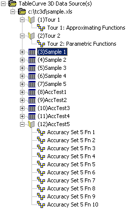
TableCurve 3D uses a Windows explorer-like approach for collecting references to data and analyses into a single notebook file. A TableCurve 3D notebook file can contain an unlimited number of references to XYZ data sets and an unlimited number of analyses. A notebook file contains references to all data items and the processing instructions for all surface-fits and other procedures used in a particular analysis.
Linked Data Sources
A TableCurve 3D notebook uses an SNB extension and stores only links to data sources already existing on disk. The actual data are not stored in the notebook file, only a reference to the file(s) and the various worksheets, columns, etc. used to specify the XYZ data tables used in the analyses. If a data table is created from within TableCurve 3D, it is saved to disk as an external file in one of the supported export formats and automatically added to the notebook.
The advantages of this linked approach is that the notebook files are very compact, and all changes made in the external data sources will be automatically reflected when subsequently opening an existing notebook.
The drawbacks involve the need to include the data source files when sharing a notebook with a colleague and the possibility of invalidating one or more analyses with external changes in the data. Moving one or more data files to a different directory will result in the disappearance of these sources from the notebook. Modifying a data source so that the size of any specified XYZ is smaller, or where it includes negative X or Y values when this was formerly not the case, can result in a notebook surface fit item becoming invalid.
tree03.png Creating a New Notebook File
The New... item is in the File menu, the main toolbar, and in the right click popup menu when on the uppermost item in the explorer. This will clear the existing notebook information, if any, in order to create a new notebook file. The TableCurve 3D explorer will have only a single empty TableCurve 3D Data Source(s) folder when a new notebook has been opened. The main window of TableCurve 3D contains the explorer, a pane containing a graph of the current data, and a pane containing the statistics for the current data or analysis. The graph and statistics will be empty when a new notebook is created, and when the item in the explorer is a folder rather than a data or an analysis item.
TableCurve 3D automatically opens with the state of the notebook session that existed when the program was last closed. Use the New item to clear this information in order to start a new notebook session.
loadsnb.png Opening a Notebook File
The Open... item is in the File menu, the main toolbar, and in the right click popup menu when on the uppermost item in the explorer. This will close the current notebook and open a new notebook file from disk. Only a single SNB notebook file can be open at any given time. A notebook file can contain as many data sources and analyses desired, and there is no limit on the number of folders or levels in the notebook. When a notebook has been opened, the uppermost folder will reflect the name of the notebook file.
savesnb.png Saving a Notebook File
The Save item is in the File menu, the main toolbar, and in right click popup menu when on the uppermost item in the explorer. It is used to save the existing notebook to disk. The notebook file will have an SNB extension. If the name for the current notebook has not yet been specified, a file name must be specified. When a notebook has been saved, the uppermost folder will reflect the name of the notebook file.
The Save As... item is in the File menu and in right click popup menu when on the uppermost item in the explorer. It is used to save the existing notebook to a new notebook file. The new SNB file name must be specified.
fileimport.png Importing a Data Source
A data source must first be imported into the notebook before it can be used. This is done via the Import Data Source item in the File menu and in the right click popup menu when on the uppermost item in the explorer. Importing a data source adds this file to the notebook and makes it available for the specification of XYZ data sets. A data source can be any of TableCurve 3D's supported file formats:
- XYZ, and Multi-column ASCII files
- Excel (XLS v3-XLS Office XP)
- Lotus 123 (WK4, WK3, WK1, WKS, WRK)
- Quattro Pro (WB2, WB1, WQ1, WKQ)
- SigmaPlot (JNB, SPW, SP5, SPG)
- XYZ, and Multi-column DIF files
- dBase III+ and dBase IV (DBF)
- SPSS Windows (SAV)
- Systat Windows (SYS)
No XYZ specification is automatically created when importing a data source. This is true even when the data source contains only a single XYZ data set, as is the case for an ASCII export of the current data.
Data sources can also be added to the notebook by dragging and dropping files from Windows Explorer into the main window.
specxyz.png Specifying Individual XYZ Data Sets
An XYZ data set is specified from a data source.
An ASCII file exported from TableCurve 3D is written in a default format that automatically defines the XYZ data, weights if present, and the current state of each triplet in the data stream. To access the XYZ data within this type of XYZ ASCII data source, click on the '+' symbol to the left of the data source folder in order to expand the item. The titles currently in the ASCII file are then presented and can be modified. Any modifications are retained in the tree only, and no modifications are made to the titles in the source file. Once the data set has automatically specified by this procedure, the titles can be accessed by selecting the data set and using the Titles option in the right click menu or in the main Table menu. The new XYZ data item is automatically selected and a surface graph using the Renka I non-parametric interpolant and the basic statistics of the data set are shown.
An Excel file or other multi-worksheet data source is also expanded by clicking on the '+' item to the left of the data source folder. For an Excel file, the names of each of the worksheets are shown as subfolders. The subfolder for the worksheet of interest must be selected in order to specify an XYZ data set from columns of data in that particular sheet. For formats that do not offer multiple worksheets, the XYZ data set specifications are done from the original data source folder.
An XYZ specification is done using the Specify XYZ Data Item in the File menu or from the right click popup menu when the data source or data source worksheet folder is selected. The specification begins with a column selection procedure and is followed by a titles option. Any modifications are retained in the tree only, and no modifications are made to the titles in the source file. Once the data set has automatically specified by this procedure, the titles can be accessed by selecting the data set and using the Titles option in the right click menu or in the main Table menu. The new XYZ data item is automatically selected and a surface graph using the Renka I non-parametric interpolant and the basic statistics of the data set are shown.
specxyz2.png Automatically Specifying Multiple XYZ Data Sets
For a spreadsheet it is possible to automatically specify all of the XYZ data sets for a given worksheet, or for the whole of the file. In order to use this feature, the data must be in a specific format. Two formats are supported. The first requires a sequence of X,Y,Z data columns. The other requires a single X and Y column followed by any number of Z columns. Blank columns and columns without numeric data are permitted and are not used in the sequencing.
To automatically specify all data sets in an Excel or other spreadsheet file, select the Excel data source before any individual XYZ specifications have been made on the file, and before expanding the Excel file to create the individual folders for the worksheets. Select the Excel data source and use the Autospecify All XYZ Data Items option in the File menu or from the right click popup menu. The XY many Z option is for the case of a single X and Y column followed by any number of Z columns. The XYZ triplet is for a repeating sequence of X, Y, Z columns. The data sets and titles are automatically created for all of the worksheets.
To automatically specify all data sets in an Excel or other spreadsheet file, expand the Excel data source to create the individual folders for the worksheets, but do not specify any individual data sets for the specific worksheet desired. Select that specific sheet and use the Autospecify All XYZ Data Items... option in the File menu or from the right click popup menu. Again, the XY many Z option is for the case of a single X and Y column followed by any number of Z columns. The XYZ triplet is for a repeating sequence of X, Y, Z columns. The data sets and titles are automatically created for this specific worksheet.
Data Items
Selecting an XYZ data item displays that data in a surface graph using the Renka I interpolant. The basic statistics for the data are also given. Clicking on the graph opens the View Data Graph option. The current settings in this option determine the display of all data items in the notebook. While it is possible to modify the titles associated with a data item, it is not possible to modify the graph settings. A new view item must be created in order to lock in specific graph customizations. The advantage of this approach is that the graphing of all data items in a notebook are updated with only one adjustment in this option.
view.png View Items
When the View Data Graph option is open from the View menu, the main toolbar, or by left clicking the graph when a data item is selected in the notebook, it is possible to Add a view item to the notebook. The view item will contain the current graph customizations and will be added to the TableCurve 3D explorer as a child of the original data item. If a view item is selected and the graph is clicked, the View Data Graph option will also offer an Update option. This replaces the current content of the view item with any revisions in the graph settings.
section.png Section Items
Any item containing XYZ data can be sectioned. This is done using the Section Data option in the View menu or main toolbar. The Add option in the sectioning creates a section item in the notebook that contains a subset of the original data and can be used just as a data item would be used. A section item is added to the TableCurve 3D explorer as a child of the item furnishing the data. If a section item is selected and the graph is clicked, the Section Data option will offer an Update option that replaces the current content of the section item with the revised sectioning as well as all graph customizations.
calc.png Calculation Items
A calculation or data transform can be applied to any item containing XYZ data. This is done using the Enter Calculation option in the Calculate menu or main toolbar. The Add option in the Undo graph that follows the application of a calculation creates a calculation item in the notebook that contains the transformed data and can be used just as a data item would be used. A calculation item is added to the TableCurve 3D explorer as a child of the item to which the calculation was applied. If a calculation item is selected and the graph is clicked, the Enter Calculation option's Undo graph will offer an Update option that updates the current calculation as well as all graph customizations.
smloess.png Smooth Loess Items
The Loess smoothing option can be used on any item containing XYZ data. This is done using the Smooth Loess option in the Table menu or main toolbar. The Add option creates a smooth Loess item in the notebook that contains the smoothed data and can be used just as a data item would be used. A smooth Loess item is added to the TableCurve 3D explorer as a child of the item that furnished the data to the smoothing algorithm. If a Loess smoothing item is selected and the graph is clicked, the Smooth Loess option will offer an Update option that updates the current smoothing as well as all graph customizations.
smnurbs.png Smooth NURBS Items
The NURBS smoothing option can be used on any item containing XYZ data, although it is primarily of value only for gridded data. This is done using the Smooth NURBS option in the Table menu or main toolbar. The Add option creates a smooth NURBS item in the notebook that contains the smoothed data and can be used just as a data item would be used. A smooth NURBS item is added to the TableCurve 3D explorer as a child of the item that furnished the data to the smoothing algorithm. If a NURBS smoothing item is selected and the graph is clicked, the Smooth NURBS option will offer an Update option that updates the current smoothing as well as all graph customizations.
flsprse.png Fill Sparse Grid Items
The Fill Sparse Grid option in the Non-Parametric menu and main toolbar is used to fill in missing values in gridded data or to form a grid that uses scattered data elements. The Add option creates a fill sparse grid item in the notebook that contains the interpolated data and can be used just as a data item would be used. A fill sparse grid item is added to the TableCurve 3D explorer as a child of the item that furnished the data to the interpolation algorithm. If a fill sparse grid item is selected and the graph is clicked, the Fill Sparse Grid option will offer an Update option that updates the current interpolation as well as all graph customizations.
ipdata.png Interpolate to Uniform Grid Items
The Interpolate to Uniform Grid option in the Non-Parametric menu and main toolbar is used to create an arbitrary density gridded data from scattered data. The Add option creates an interpolate to uniform grid item in the notebook that contains the interpolated data and can be used just as a data item would be used. An interpolate to uniform grid item is added to the TableCurve 3D explorer as a child of the item that furnished the data to the interpolation algorithm. If an interpolate to uniform grid item is selected and the graph is clicked, the Interpolate to Uniform Grid option will offer an Update option that updates the current interpolation as well as all graph customizations.
estgrid.png Estimate Gridded Data Items
The Estimate Gridded Data option in the Non-Parametric menu and main toolbar offers spline interpolation and smoothing. The Add option creates an estimate gridded data item in the notebook that contains the output of the spline estimation. This procedure is treated as producing a continuous surface rather than discrete data and cannot be subsequently processed. An estimate gridded data item is added to the TableCurve 3D explorer as a child of the item that furnished the data to the non-parametric algorithm. If an estimate gridded data item is selected and the graph is clicked, the Estimate Gridded Data option will offer an Update option that updates the current estimation as well as all graph customizations.
estscat.png Estimate Scattered Data Items
The Estimate Scattered Data option in the Non-Parametric menu and main toolbar offers non-parametric interpolation and smoothing. The Add option creates an estimate scattered data item in the notebook that contains the output of the non-parametric estimation. This procedure is treated as producing a continuous surface rather than discrete data and cannot be subsequently processed. An estimate scattered data item is added to the TableCurve 3D explorer as a child of the item that furnished the data to the non-parametric algorithm. If an estimate gridded data item is selected and the graph is clicked, the Estimate Scattered Data option will offer an Update option that updates the current estimation as well as all graph customizations.
grsrt.png Graph Start Surface Fit Items
The Surface-Fit Review is the point where surface fit equations are added to the notebook. If the Review is started with the Graph Start option, the Add option in the Review creates a graph start surface fit item in the notebook that contains the fitted equation currently being inspected. This procedure is treated as producing a continuous surface rather than discrete data and cannot be subsequently processed. A graph start surface fit is added to the TableCurve 3D explorer as a child of the item that furnished the data to the fitting algorithm. If a graph start surface fit item is selected and the graph is clicked, the data will be refitted using the fit preferences and equation set in place at the time of the previous processing. The equation list will reproduce the previous one, provided the target data is unchanged. In this instance, the Surface-Fit Review offers an Update option that updates the current equation as well as all graph customizations. The equation in the update need not be the same as prior.
lsstr.png List Start Surface Fit Items
If the Review is started with the List Start option, the Add and Update options in the Review function similarly except that a list start surface fit item is crated.
tree18.png Annotation Items
The File menu's Add Annotation option is used to open an ASCII text editor. ASCII files can be imported, or the text can be added within this editor. Use this option to add experimental notes, observations, methodology notes, and other information pertinent to the current notebook. The annotation item is automatically created when the ASCII editor is closed. Unlike the data items, which use links to data sources, annotations are stored locally within the SNB notebook file. Also, unlike the other items in a notebook, annotations are displayed exclusively in the main statistics pane.
Adding Multiple Analyses
From any procedure, the Add option can be used as many times as desired to create multiple notebook items that reflect various surface-fit equations, graph settings, algorithms, and algorithm parameters.
Updating the Analysis
Since all data is stored externally, and a notebook file consists only of references or links to these files, an update will automatically occur each time the external data source is accessed. TableCurve 3D does not scan for changes in referenced files, so the current data item or any subitem of the currently selected data will not be updated when the external source itself changes. However, the update will occur the next time that data item or any subitem is selected.
Deleting Items
The Remove Selected Item in the File menu and right click popup menu will delete the current item in the notebook and all subitems that are based upon the item being removed.
Renaming Items
The Rename Selected Item in the File menu and right click popup menu is used to rename the current item in the notebook.
Exporting a Data Item
Any item containing XYZ data can be exported. The Export XYZ option in the File menu is used to save the current XYZ data set to a file.
Drag and Drop, Copy and Paste
Certain operations can be copied and pasted, or dragged and dropped, from one item to another. If the selected item represents an operation on an XYZ data set that results in XYZ data, it can be dragged or copied to any XYZ item in the notebook. When a component is bring dragged, the cursor will change reflect whether or not the first item can be dropped on the item at the cursor.
This operation can be done most easily using the mouse, although the File menu contains a Copy Item and Paste Item option. The standard copy (Ctl-C) and paste (Ctl-V) shortcuts can also be used.
As an example, a smoothing item can be dragged from its current position to any target item containing XYZ data in order to create a new smoothed data item.
Appending Data Sets
When one XYZ data set is dragged upon another, an Appended Data folder is created and a new XYZ data item is created in this folder. The new data item represents the result of appending the two sets. It is possible to create as many appended sets as desired, and to append individual data sets to a set in the appended folder. This approach can be used to quickly create sets which reflect the combination of many individual sets, without storing the appended set to disk.
Special Import Operations
TableCurve 3D offers three special Import Special procedures in the File menu.
- The Import Clipboard option converts the clipboard contents to an ASCII or spreadsheet file and automatically adds this new file as a data source.
- Similarly, the Import Clipboard Matrix option converts an XYZ data matrix on the clipboard to an XYZ ASCII data file and adds this file to the notebook.
- The Import Digital Filter option is used to set intrinsic filter settings for the import of all data streams.