Exploring Surface Fitting Pitfalls
The purpose of this section is to illustrate some of the pitfalls that exist in surface-fitting science, and some of the ways they can be avoided. TableCurve 3D contains a significant number of features designed explicitly to prevent the kind of errors that are common to surface-fitting.
Partial Extrapolations
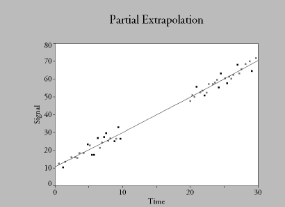
While partial extrapolations are not unique to 3D surface-fitting, they are found far less frequently in 2D curve-fitting. It is fairly obvious, for example, that there is something profoundly incomplete about the 2D data fitted below. For this curve to be a reliable estimator across the X range of data, it is obvious that there has to be some data in the middle of the X range. Estimations in this data-barren region are partial extrapolations.
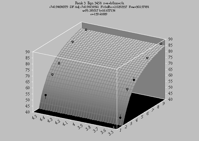
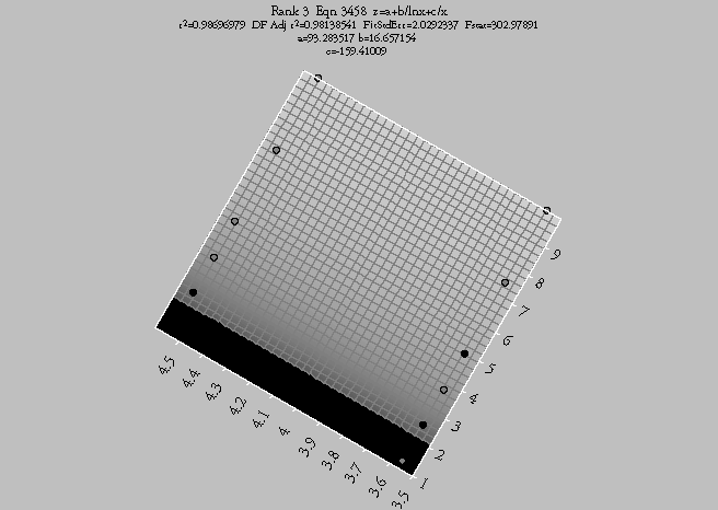
In 3D surface-fitting, you should try to collect data for the whole of the 2D space defined by the range of X and Y variables. On first inspection, this fit would seem to be valid. A 90 degree Z view angle, however, makes it readily apparent that a partial extrapolation is taking place for most of the surface:
Full Extrapolations
Unlike 2D curve-fitting, it is possible to see full extrapolation within the range of X,Y data. This often occurs where there is a relationship between the X and Y variable which constrains the range of viable data. Consider this data set which is fitted well by one of TableCurve 3D’s simple equations:
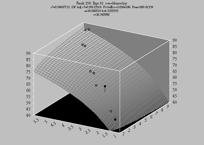
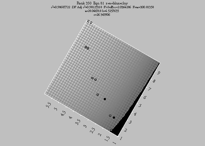
Here the XY zone defining the surface is less than 5% of the overall area formed by the X and Y ranges. Anything outside this narrow region of definition is a full extrapolation, even though both the X and Y value may be within the X and Y range of the data table. Such extrapolations are every bit as dangerous as those which lay outside the X and Y ranges. In fact, the extrapolated Z at [11,6] is likely to be more reliable than the extrapolated Z at [6,2] even though the latter is within both the X and Y data ranges, and the former is not.
The best way to be certain of the bounded region of data where interpolations can be safely inferred is to use a 90° Z view angle or a contour plot.
Rational Equations
Rational equations consist of the ratio of two polynomials as in the following examples:
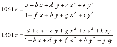
The first equation contains no X-Y interaction term while the second contains an interaction term in both the numerator and denominator.
Although the first type of equation contains no interaction terms, such equations are still very capable of modeling X-Y interaction. This is because the whole rational equation is one giant interaction term—the X-Y interaction being intrinsically a part of the division.
As such, 3D rational equations tend to be very good at fitting data containing X-Y interaction. They are not particularly good models for approximating data where this interaction is absent.
The following example illustrates an effective use of a 3D rational surface-fit. The essential elements for 3D rational fitting are:
- X-Y Interaction
- Accurate Data Relatively Free of Noise
- Observations at All Points within an XY Grid
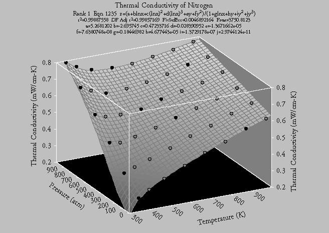
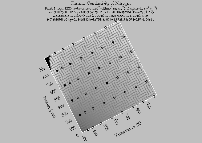
While this fit is very effective, 3D rational equations have very definite drawbacks. Because rational equations consist of the ratio of two polynomials, there is the danger of such functions becoming unstable or undefined as the polynomial in the denominator approaches a zero value.
Such unstable regions exist where the surface suddenly sweeps off the top or bottom of the plot, and then reappears nearby, possibly from the opposite direction. Also, a small spike is usually indicative of such an unstable region.
In surface-fitting, it may be necessary to expand the resolution of the underlying grid to see these effects. It may also be of value to use a shaded plot. The following example illustrates the value of a higher resolution shaded plot in detecting these unstable regions:
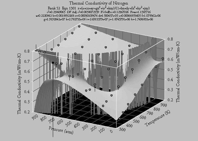
This plot uses a 120x120 grid with a 60° Z illumination angle. Note how the singularity winds through the 3D surface.
Extrapolating Rational Functions
Whenever you are dealing with partial or full extrapolation, you should not even think of extrapolating a 3D rational equation without first carefully zooming out the surface and performing a rigorous visual inspection.
It would be a grave mistake to extrapolate a rational function blindly, even if the X,Y data is only slightly outside the bounds of the original data.
To illustrate this point, consider the excellent rational fit shown on previous page. A single level of zoom-out on the X and Y ranges of the plot reveals the following:
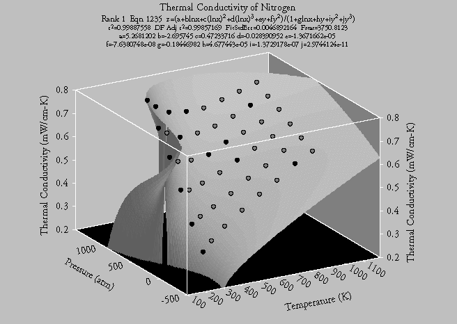
Note the one region very nearly at the bounds of the data where the surface folds into a singularity band. This is not at all uncommon behavior with 3D rational equations.
In general, extrapolating a two dimensional curve is highly risky. When it comes to three dimensional surfaces, you must be able to anticipate the trends in both the X and Y variables as well as any interaction between them. It is our view that consistently successful 3D extrapolations can come only from genius or a great deal of good fortune, neither of which tend to be particularly common.
Extrapolating Polynomials
The dangers and pitfalls of extrapolation are traditionally demonstrated with higher order 2D polynomial equations. Such curves tend to wander off into seemingly random oblivion the moment the curve is outside the data.
In 3D surface-fitting, blindly extrapolating higher order 3D polynomials is equally an exercise in analytical suicide. For example, consider a modest zoom-out of two different Taylor polynomial fits to this same data set:
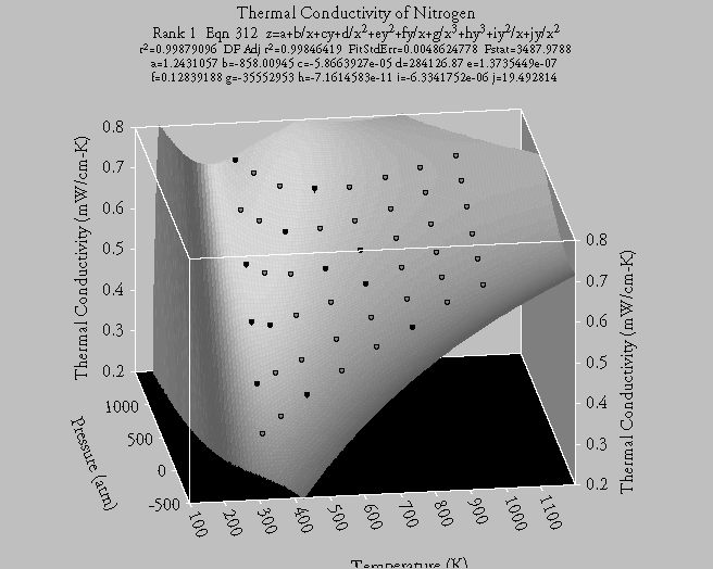
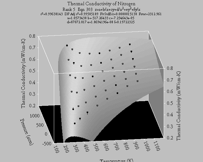
Note how foolhardy any extrapolation would be to lower temperatures. In this example, the equation in the first plot is actually a higher order expansion of the model in the lower plot.
Extrapolating polynomials and rationals isn’t necessarily impossible. It should, however, be considered an art requiring a great deal of caution and no small measure of judgment and insight as to expected trends.
Understanding Interaction
One of the confusing concepts surface-fitting introduces is the idea of interaction and non-linear profiles. In the 2D curve-fitting world, a Gaussian peak is a single function, with an easily recognizable profile. With 3D surface-fitting, there is no such thing as a single 3D Gaussian peak. There are rather a variety of profiles:
Function in One Variable
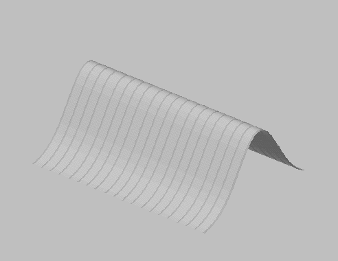
Multiplicative - Full Interaction
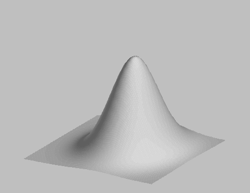
Additive - No Interaction
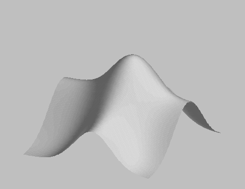
Multiplicative and Additive - Synergistic
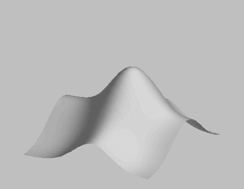
All four of the surfaces consist of 3D Gaussian functions. The difference is within the profile or interaction. In the first instance, the Gaussian behavior is evidenced in only one of the variables, and there is no interaction. In the next three plots, the Gaussian behavior applies to both the X and Y variables. In the second plot, the interaction of both variables determine the the function. In the third plot, there is no interaction—the Gaussians in each dimension are summed to produce the surface.
In the last plot, both types of behavior are present. A synergistic model offers a measurement of the independence of the variables, as well as a means to quantify the interaction. If the interaction term is positive, there is a positive synergy. If the interaction term is negative, there is a negative synergy or antagonism.
If you are seeking to discover or develop a 3D surface model for a given physical process, you must have some means of formulating the independent effect of each variable as well as the interactive effect.
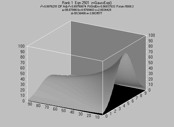
Also in terms of profiles, it is important to bear in mind that the X and Y variables might require entirely different non-linear base functions. For example, a profile might be Gaussian in one variable, and a first order kinetic decay in the other:
Robust Fitting
In the following example, noisy plane data is fitted by least squares and by TableCurve 3D’s medium robustness procedure, that which assumes Lorentzian errors.
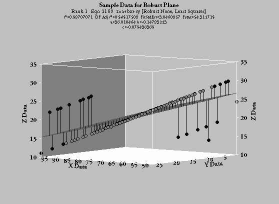
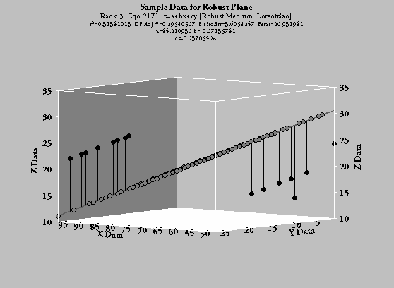
Note also the value of adjusting view angles. In these plots, the view angles have been adjusted so that all of the points forming the bulk of the plane appear as a line, making it easy to see the degree to which the outliers influence the overall fit. Note also that the robust fit in the lower plot has poorer goodness of fit statistics than the least-squares fit in the upper plot.
Since robust methods assume a wider distribution of errors, such fits are far less impacted by the outliers.
You should use TableCurve 3D’s robust fitting procedures when you are fitting a non-linear model (or are willing to fit a linear model by a UDF), and one or more of the following are true:
- The data spans many orders of magnitude in Z and the low-valued Z points are not factoring into the least-squares fit.
- The distribution of residuals is likely to have broader tails than that of a Gaussian distribution.
- The data is noisy, outliers are suspected, but excluding these outliers is not straightforward.
Numeric Indices Of Fit
Numeric goodness of fit values will never reveal unstable or undefined regions within a surface unless the singularity occurs near or at one of the data points. In a least-squares surface fit with a wide dynamic Z range, the low Z-value points may factor quite poorly into the fit without any indication of a problem in the goodness of fit statistics. A robust fit may fare far better in fitting the bulk of the data, eliminating the impact of outliers, but goodness of fit statistics will not reflect this.
We cannot stress strongly enough how crucially important it is that you visually inspect the candidate surface-fits before selecting the one you will use within your work. TableCurve 3D furnishes a host of tools to assist you. Use high-resolution plots to detect unstable or undefined regions. Use gradient or shaded plots to see the nuances in the surface. Use the SD coloring of points, residuals plots, and intervals to detect outliers. Zoom out the surface-fit graph before you even consider the possibility of extrapolations.
While software can place powerful tools are your fingertips, surface-fitting is still an art in terms of selecting the model most appropriate to your data. Numeric statistics should be used only to suggest possible fits. Your own knowledge of the data, your insight of the problem, and your own analytical judgment should be the final determinant.