Approximating Functions

Tutorial 1: Approximating Functions

An approximating function is an equation that is used to represent X,Y,Z data. An approximating function can be used for interpolation, finding a Z-value for an X-value and Y-value within the range of the data. An approximating function can also be cautiously used for extrapolation, the process of finding a Z-value for an X-value and Y-value where one or both lie outside the range of the data.

Approximating functions can be differentiated or integrated, both numerically and analytically, resulting in far more accurate computation of volumes under surfaces, minima and maxima, and other analytical elements than would be realized by working with the raw data. An approximating function is also the finest form of data smoothing in the time domain.

What is important in an approximating function is seldom the coefficient values derived from the fit, but rather the effectiveness of the fit itself. Equally, the number of coefficients is of minor importance. For this reason, linear models are most frequently used for approximating functions. In the example that follows, we will only be surface-fitting linear models.

Adding a Native XYZ Data Item to the TableCurve 3D Notebook

Starting TableCurve 3D

Start TableCurve 3D by selecting TableCurve 3D v4.0 from the Start menu.

If the existing notebook is not empty, select New from the File menu.

z = f(x,y)

In TableCurve 3D, the dependent variable is Z. All equations express Z as a function of the two independent variables X and Y. For all built-in equations, X and Y are interchangeable. In some manner, an individual vector of X, Y, and Z values must be specified in order to define an XYZ data table.

Setting up an XYZ Data Table

The first step in using TableCurve 3D is to set up an XYZ data table. TableCurve 3D offers a maximum data table size of 16384 XYZ triplets. For larger data streams, a digital filter can be used where up to 16 million values can be filtered into the program in a single step.

Data Sources

TableCurve 3D supports the following data sources:

• XYZ, and Multi-column ASCII files
• Excel (XLS v3-XLS Office XP)
• Lotus 123 (WK4, WK3, WK1, WKS, WRK)
• Quattro Pro (WB2, WB1, WQ1, WKQ)
• SigmaPlot (JNB, SPW, SP5, SPG)
• XYZ, and Multi-column DIF files
• dBase III+ and dBase IV (DBF)
• SPSS Windows (SAV)
• Systat Windows (SYS)

For this tutorial we will use an Excel XLS file as the data source.

Importing a Data Source

Whether a data source contains a single XYZ data set or thousands, the first step is always the same. The data source must be added to the TableCurve 3D notebook.

Select the Import Data Source option from the File menu, from the main toolbar, or from the right click popup menu of the root or uppermost node of the TableCurve 3D Explorer tree in the left pane of the main window.

Click the Files of Type drop-down button and select Excel [xls] files. Select the file sample.xls and press Open.

Click the expand symbol to the left of the Excel data item.

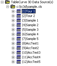
We will be specifying an XYZ data table using the columns present on the first sheet in the XLS file. There are a number of ways to initiate this process:

• left click the expand symbol to the left of the (1)Tour 1 sheet item
• double left click the (1)Tour 1 item
• right click the (1)Tour 1 item and select Specify XYZ Data item from the popup menu
• left click the (1)Tour 1 sheet to highlight it and then select Specify XYZ Data Item from the File menu
• left click the (1)Tour 1 sheet to highlight it and then click the Specify XYZ Data Item button in the main toolbar

Specifying the X, Y, Z, and Weights data columns

Click the Specify XYZ Data Item button in the main toolbar.

TableCurve 3D lists the string data existing in the first 100 rows of the spreadsheet for aiding in the identification of the columns. There must be at least one entry within the first 100 rows of a column in order for that column to be available for selection.

Select the column with the label (1)Tour 1!A Tour 1: Approximating Functions to be used as the X-variable. Select the column identified as (1)Tour 1!B Pressure(atm) for the Y-variable. Select the column with the label (1)Tour 1!C Thermal Conductivity (mW/cm-K) as the Z-variable. Check the Import Preview box to view an animated non-parametric surface of the data to be imported.

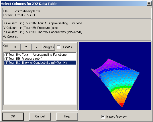
Note that the first three selections are automatically placed in the X, Y, and Z positions. To automatically select the three adjacent columns in a single step, double click the column for the X variable. To revise the initial X,Y,Z selections or to optionally specify a column to be used for weights, click the X, Y, Z, or Weights button after selecting a column. The weights can be entered as floating point multipliers or as standard deviations from averaged observations at identical X,Y values.

Press OK to accept these choices.

Default XYZ Titles

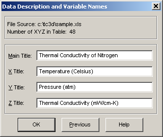
Enter Thermal Conductivity of Nitrogen for the main title.

We will accept the column titles in the spreadsheet for the X,Y, and Z variables.

Press OK to confirm these titles and create a new data item in the TableCurve 3D Explorer.

These are the default titles for this particular XYZ data item. These titles are used throughout TableCurve 3D's various procedures. These are stored within the TableCurve 3D Explorer with the data item with which they are associated.

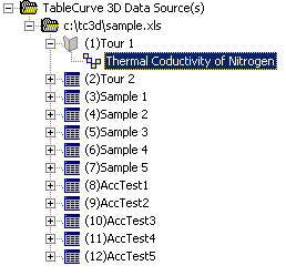
The title of the data item in the TableCurve 3D explorer will be this main title. The main title can also be edited in place directly by clicking on the item after it is already highlighted.

These default titles can be subsequently changed at anytime using the Table menu’s New Titles option, the button in the main toolbar, or by right clicking the specific data item and selecting Titles from the popup menu.

Note that the graphs incorporate these titles only as defaults. A more extensive custom titles option is available in the program’s 3D graphs.

Main Window Graph and Statistics

Non-Parametric Surface Graph

The upper right pane contains the main window graph, a non-parametric surface rendering of the data.

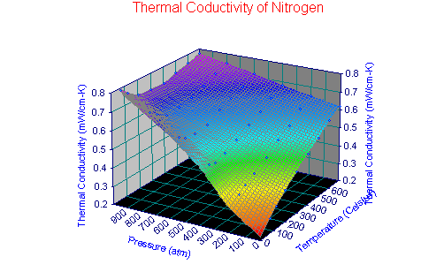
The main graph's display will depend on the object currently selected in the TableCurve 3D Explorer. For a native data item, an interpolated surface is rendered. The TableCurve 3D procedure associated with the object is opened by clicking the graph. We will do so after exploring the animation of this graph.

Select the View menu's Animation Setup item or the equivalent button in the Process toolbar.

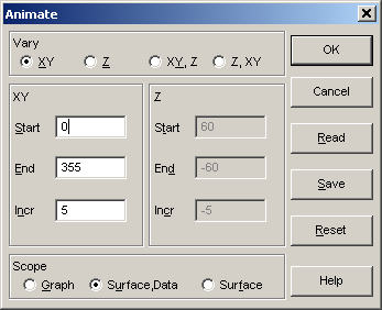
Be sure the current settings specify XY rotation, starting at 0 degrees and continuing to 355 degrees at an increment of 5 degrees, and a scope of animation consisting of the Surface,Data. Click OK.

The animation in the main window is very helpful for surface visualization. The animation can remain on while changing items in the notebook.

The animation is toggled on and off using the Animation item in the View menu or the far right button in the Process toolbar.

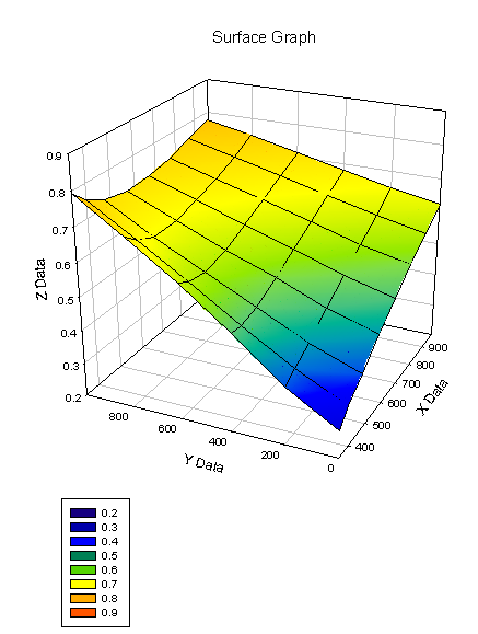
It is readily apparent that the thermal conductivity generally increases with increasing temperature and pressure.

Click the Animation button to stop the animation.

Statistics Summary

The lower right pane contains the main window statistics, a summary that is specific to the type of object selected. For intrinsic data nodes, this pane will display the basic X, Y, and Z statistics of the data table.

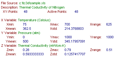
Adding Implicit XYZ Items

An implicit data item is any non-native XYZ data item created by the Add item in a TableCurve 3D procedure. We will start with a View item, a child item of a native data set that contains exactly the same data, but different graph customizations.

Click the main window graph.

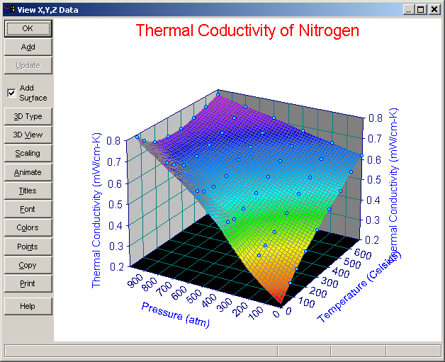
The View menu's Data Graph option opens since this is the corresponding procedure for all native data items.

Place the cursor on a data point and note the display of the X,Y,Z values.

The 3D Type, 3D View, Scaling, Animate, Titles, Font, Colors, Points, Copy, and Print items in the button panel are common to TableCurve 3D graphs containing surfaces and data. It is safe to experiment with these options. In dialogs involving adjustment options, a Reset button enables the restoration of the default settings. All adjustment options are designed to furnish immediate graphical feedback.

Unlike all implicit and output items in the notebook hierarchy, native data nodes do not contain their own graph settings. Instead the surface graph is displayed in the main window using the most recent settings in the Data Graph option. These settings are automatically updated each time the Data Graph procedure is invoked.

To change the 3D graph for all native data items, simply highlight any intrinsic data item, open the Data Graph option, change the settings, and exit the procedure. All native data nodes will now display at the new settings.

At this point, we will add a few implicit data items that represent graph customizations. We will create three new view items in the notebook: a photorealistic shaded surface, a contour plot, and a surface plot containing contours.

Photorealistic Shaded Surface

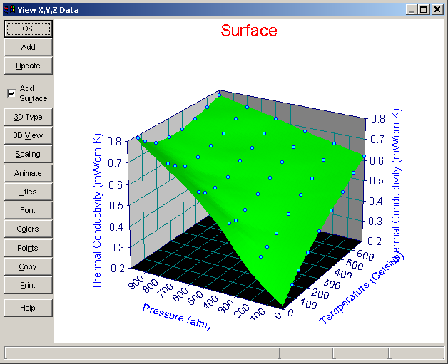
Even though a continuously increasing surface in X and Y is better suited to a gradient plot, we will create a high resolution (photorealistic) surface with light shading.

Click 3D Type. Explore the different types and finally select 160 Green in the Shaded Plots. Click OK.

Click 3D View. Explore all of the different options.

When working with View Angles, it may be helpful to imagine the surface as being fixed in space, and that you, as the viewer, freely move about a large boom that pivots about the center of the displayed surface. The XY view angle is then the angle of the projection of this boom onto the XY plane, and the Z view angle is then the angle between the boom and the XY plane.

To keep a constant reference for residuals, graphs are not shrunken or enlarged when changing view angles. The Size in Frame scrollbar must be used to shrink or enlarge the plot.

When working with Illumination Angular Shifts for shaded plots, note that these angles are specified relative to you as the viewer. The default XY shift of +30° and Z shift of +15° is somewhat analogous to holding a flashlight to your right and above your head, pointing directly at the center of the surface. Relative to the boom analogy, the illumination source is attached to the boom with a horizontal extender that shifts the source the specified number of degrees left or right, and then with a vertical extender that shifts the source the specified degrees up or down.

The Grid Level specifies the amount of interleaved space relative to the dots comprising the grid line. A level of zero is a simple line. Levels of one and above are drawn more slowly than lines.

Click Reset. Enter 250 for the Mesh Count. Click OK.

Click Add to add this 3D graph to the notebook.

Contour Plot

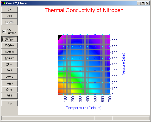
Click 3D View. Click Reset. Slide the scroll bar below the graph to a position that corresponds with an XY View angle of 270 degrees. Slide the scroll bar on the far right of the graph upward to the topmost position, this corresponding with a Z View angle of 90 degrees. Set the Perspective to Level 0. Set the Size in Frame in the scroll bar to the top of the graph to 0.80. Click OK.

Click 3D Type and select Full Spectrum. Click OK.

Click Add to add this 3D graph to the notebook.

Surface Plot with Contours

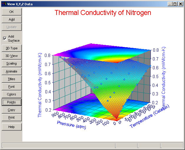
Click 3D View. Click Reset. Check both Top and Bottom under Add Contour. Set the Z View Angle to 12 degrees. Click OK.

Click Points. Explore the various options and then Click Reset. Select Visible Only. Click OK.

Click Add to add this graph to the notebook.

Click 3D View. Click Reset. Click OK.

Click Points. Click Reset. Click OK.

Click OK to exit and return to the main window.

Three new items have been added to the notebook. All contain the same icon as the toolbar button for the Data Graph option.

Select each of the items to view the associated graph. Initially, the three graphs will have the same names as the parent data. Highlight each of the three items in the tree and then click again, editing the titles in place. Name them Surface, Contour, and Surface+Contour.

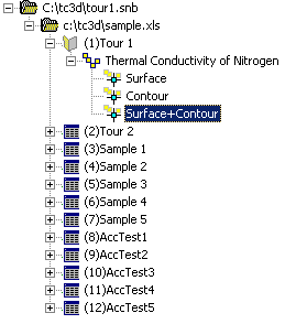
Note that the only difference between the parent data set and three child items is in the graph customizations. All four contain exactly the same data and can be used interchangeably as the source of XYZ data for surface fitting or for other procedures.

Adding a Calculation Item

Calculation

In TableCurve 3D, a data transform is known as a calculation. TableCurve 3D’s Calculate menu offers an Enter Calculation option. Use this option to transform one or more of the data vectors or to apply a weighting scheme to the whole table.

Let us assume we need an approximating function based on temperature in °K rather than °C. We will now enter a calculation to convert the Centigrade temperatures to the absolute Kelvin scale.

Select the parent data set (the one labeled Thermal Conductivity of Nitrogen).

Use the Calculate menu’s Enter Calculation item and enter X+273.15 on the X= line.

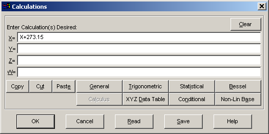
Click OK and then answer Yes to immediately apply the calculation to the existing data table.

Undo Graph

TableCurve 3D’s Undo graph appears. This type of graph allows graphical inspection of calculations before accepting the modifications. To distinguish this item in the explorer, we will generate a gradient surface.

Click 3D Type and select 64 Blue to Red. Click OK. Click Add to add this Calculation item to the current notebook.

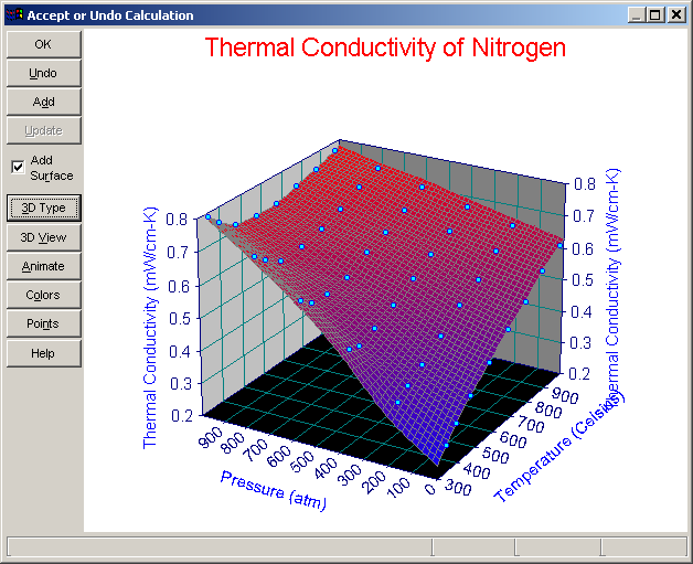
Clicking Undo returns the Calculations dialog for making revisions to the calculation expression(s). In this manner it is possible to easily add a series of different transforms to the notebook.

Click OK to exit the procedure.

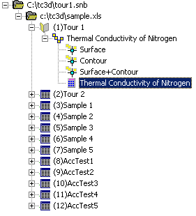
Select the new Calculation item in the notebook. The graph shown will reflect absolute temperature. Right click this item and select Titles from the popup menu. Change the X Title to reflect Kelvin rather than Celsius temperature. Click OK to close the Titles dialog.

Adding a Section Item

Individual Point State Sectioning

TableCurve 3D offers two ways to create a Section item. These implicit items are used to build an XYZ data set that is in some manner a subset of the parent data. There are two types of sectioning, setting the state of individual points and numeric range sectioning.

Individual points can be toggled on and off in the Data Graph option and in the Section Data option. Either option can be used to create this type of data object.

To graphically toggle individual points between an active and inactive state, place the cursor directly on a data point. A special cursor will show that a point is contained inside and the information display below the graph will indicate the point detected and its status. To change the status of the data point, simply click and release the left mouse button. The point's color will change to reflect its new status.

Be sure the new Calculation item is highlighted in the notebook (the graph shown will reflect Kelvin temperature).

Click the Data Graph button in the main toolbar. Click several points off and then click Add, and then click OK.

There is now a Section item in the notebook that contains a subset of the original XYZ data.

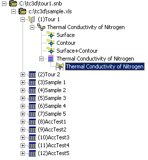
Select the new Section item and observe the inactive points in the graph.

The points that were toggled off are rendered in the color assigned to inactive points. These points are not used in surface fitting.

Numeric Range Sectioning

Select the Calculation item to highlight it and then click the Section Data button in the main toolbar.

Here we will construct a low temperature, low pressure data extract.

Enter 300 for the initial X value and 700 for the final X value. Enter 0 for the initial Y value and 500 for the final Y value. Be sure Include is checked. Click Apply New.

All of the data values between 300 and 700 degrees Kelvin and 0 to 500 atmospheres comprise this subset.

Click 3D Type and select 64 Green to Blue. Click OK.

Click Add to add this Section item to the notebook. Click OK to exit the Section procedure.

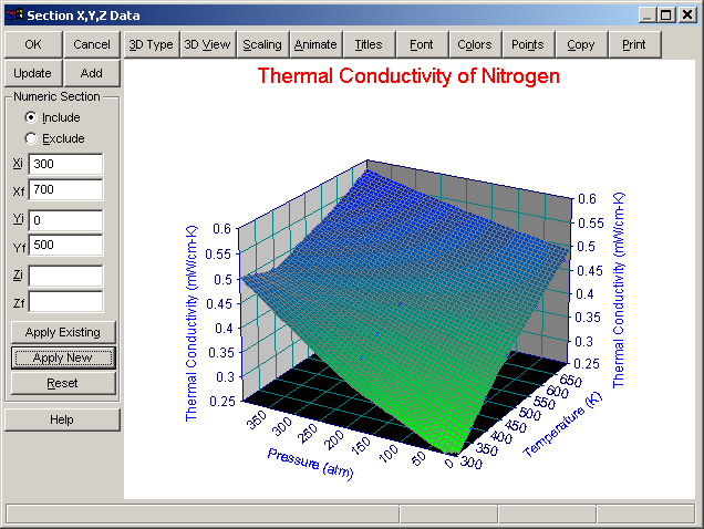
Select this Section item and observe the same reduced range plot in the main window graph.

Adding a Smooth Item

The Smooth Loess option is TableCurve 3D's principal smoothing procedure. It offers an effective nearest neighbor Loess (locally-weighted regression) type of smoothing. This procedure works equally well with scattered or gridded data.

Although this data set has no need of smoothing, we will create several smoothing items.

Select the parent data set (the one labeled Thermal Conductivity of Nitrogen).

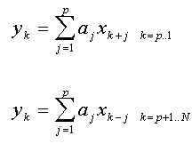Select the Smooth Loess item in the Table menu or in the main toolbar. Set the order to 1 and the count to 24. Click Add.

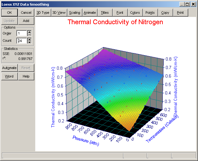
This represents a very high level of smoothing.

Set the order to 2 and the count to 12. Click Add.

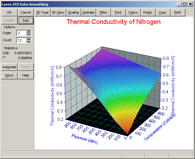
This represents a very modest level of smoothing.

Click OK to exit the Loess procedure.

Dragging and Dropping Analysis Items

We will now copy these smoothing objects to different data nodes. We will be copying the smoothing objects to data nodes containing the same XYZ data.

Drag the first of the two Loess smoothing items to the first of the section objects.

Highlight the second Loess smoothing item and click the Copy Item button in the main toolbar.

Select the data node with the calculation icon and click the Paste Item button in the main toolbar.

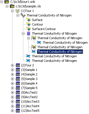
This is an easy way to apply a given analysis across a number of XYZ data sets.

Adding Non-Parametric Estimation Output

There are two types of output items in a TableCurve 3D notebook. These are the non-parametric and parametric fits. We will begin by adding Non-Parametric Estimation objects.

Highlight the data node with the calculation icon and click the Estimate Gridded Data button on the main toolbar. Select the Bicubic+Akima algorithm which supports extrapolations. Click Add.

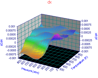
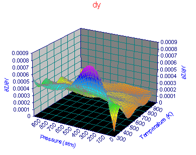
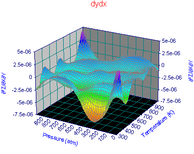
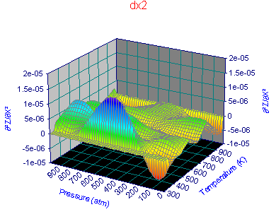
Select the dX Partial Derivative and click Add. Select dY and click Add. Select dXdY and click Add. Select dX² and click Add. Select dY² and click Add. Click OK.

For these six items, edit in place (or right click and rename) as follows: Fn, dx, dy, dydx, dx2, dy2.

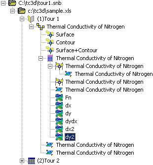
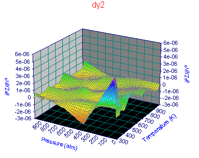
Select the six new output objects. The following graphs are shown in the main window when selecting these six items:

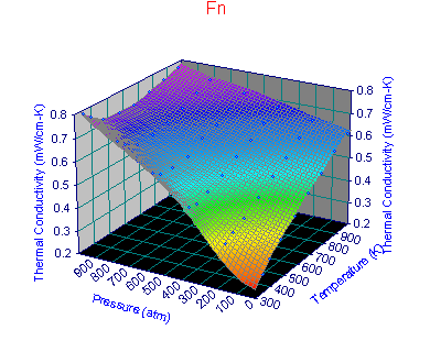
Adding Surface Fit Equations

The Surface-Fit Processing

The TableCurve 3D linear engine processes the data table fitting up to 310 XY polynomials, 300 XY rationals, and up to 36,582 selective subset equations from a total set of 453,696,714. This fitting is fully automated and occurs in a single step. In this tutorial, we will fit the thermal conductivity data to all of TableCurve 3D’s linear equations.

To view a list of the TableCurve 3D equations, use the four List items in the main Help menu.

Fitting Speed

Because of the numerically intense nature of this processing, the time required for the fitting that follows will vary in relation to the computer’s floating point performance. A Pentium machine should require only a few seconds to fit all linear equations to the data used in this tutorial.

Customizing TableCurve 3D’s Surface Fitting

TableCurve 3D has two levels of customization, one that sets surface-fitting preferences and the other that offers a custom equation set.

The Process menu option Edit Custom Equation Set offers the means to select particular linear families of equations and specific non-linear types and profiles to be fitted. These selections affect only the Surface-Fit Custom Equation Set fitting option.

The Surface-Fit Preferences option in the Process menu consists of specific fitting controls that are applied to every TableCurve 3D fit.

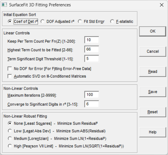
Highlight the data node with the calculation icon and then select the Process menu’s Surface-Fit Preferences option. Select the DOF Adjusted r² option in the upper section of the dialog.

This initially sorts the fitted equations by a degree-of-freedom adjusted coefficient of determination. For approximating functions, the equations can be sorted by the DOF Adjusted r² or by the Fit Std Error, both of which take into account the degree of freedom in the fitting.

Keep Best

This is one of the most important controls in the program. This value determines how many of the fitted equations are preserved for the Review. This count is based upon equation type, term count, and Z-transform. A Keep Per Term Count Per Fn(Z) of 10 means that TableCurve 3D saves up to 10 standard polynomials of each term count, up to 10 standard rationals of each term count, and up to 10 selective subset equations for each term count and Z-transform. Specialty series equations, such as Chebyshev, Fourier, Cosine, and Sigmoid models, are always added to the equation list when successfully fitted.

Other Linear Controls

Linear controls include the Highest Term Count to be Fitted and Term Significant Digit Threshold items. A maximum term count of 66 accommodates all of TableCurve 3D’s equations. A term significance of 5 means that an equation is added to the list if each of its terms essentially makes at least a 1E-5 fractional contribution to the Z value. The No DOF for Error should be used only for fitting error-free handbook data. The Auto-SVD option fits saved equations by the SVD method, and if a better least-squares solution is found, this solution will replace that produced by the standard matrix procedure. The Auto-SVD option does not apply to specialty series equations (Chebyshev, Fourier, Cosine, and Sigmoid).

Non-Linear Controls

While we will not be fitting non-linear equations in this mini-tour, this is a good point to take note of the two principal non-linear fitting controls. Non-linear fitting is iterative, and as such, the maximum number of iterations permitted for a non-linear equation, as well as the convergence criteria, are selectable. The default Maximum Iterations of 100 should be sufficient for all except highly complex UDFs with poor starting estimates. The default Converge to Significant Digits in r² of 6 means that the r² must be unchanging in the sixth significant figure for 5 consecutive iterations to signal convergence.

Starting the Surface-Fit

In this tutorial we will not be fitting a custom equation set. Press OK to close the surface-fit preferences. Select the Process menu option Surface-Fit Linear Equations. This begins the automated surface-fit processing for all linear equations.

During the linear fitting, the automated processing can be aborted at anytime by clicking on the Cancel button.

There is first a sums generation followed by the polynomial fitting, the rational fitting, and finally the Z, ln Z,and 1/Z selective subset fits. The ln Z and 1/Z selective subset fits are terminated early for this data set, since these transforms produce fits that are inferior to the standard Z subset fits.

The Surface-Fit Review

When the automated fit is concluded, equations with insignificant terms have been removed and the set has been sorted by the specified goodness of fit criteria. The equation at the top of the list, #424, a Chebyshev bivariate polynomial, is pre-selected.

If the default fitting controls have not been modified, 14446 equations were fitted and the best of these were saved to the Review list.

Select Graph Start to begin the Review.

Note: If there is no response to the conclusion of the fit in 10 seconds, the Review is automatically started.

An alternative consists of clicking OK and then selecting the Graph Start item in the Review menu.

The List Start and Graph Start options represent two different desktops for a single Review process, the primary difference being that the equation list will close after each selection when the List Start option is used to begin the Review.

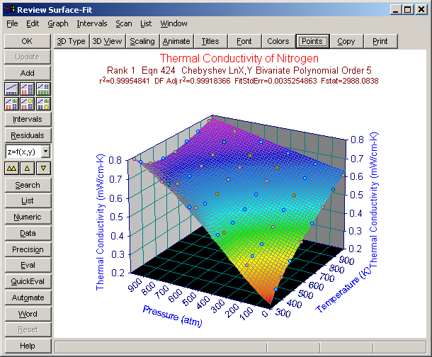
Click the button for the simplest of the automatic tiling options. The Surface-Fit Graph and Equation List are automatically opened and positioned.

Selecting an Equation

We will now choose from amongst the candidate equations to select the one best suited to this application. Note that the Surface-Fit graph consists of a plot of the highest ranked equation.

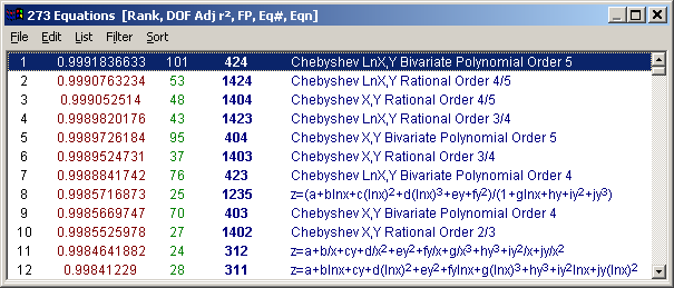
The equation list contains the best 263 equations from the thousands that were fitted. For this particular data set, Chebyshev and standard polynomial and rational equations are clearly the most effective approximating functions.

Floating Point Speed

In the equation list, there is an FP column containing the estimated floating point execution speed. This value is based on TableCurve 3D’s code generation and is derived from assigning a value of 1 to a floating point addition. An equation with an FP of 45 should require about three times as long to execute as one with an FP of 15. For this data set, there are significant differences in execution speed amongst the best equations. In particular, the Chebyshev series models require appreciably longer to execute than conventional polynomials or rationals.

Inspecting the Various Equations

To view the surface-fit graph for other candidate equations, use the arrow buttons in the Surface-Fit graph’s control panel or select the equation directly from the equation list. The arrow buttons are particularly useful when the equation list window is not currently displayed.

Use the arrow buttons to move about the initial equations. Similarly, use the direct selection method within the equation list to view these initial equations.

Click the Add button after selecting each of the first three equations in the list. Use the double upward arrow button to return to Equation 424, the highest ranked equation by DOF-adjusted r².

Note that points are colored by standard error by default. Yellow points lie outside ± 2 standard errors of the overall fit while the red points lie outside ± 3 standard errors.

Automatically Tiling Windows

Explore the various buttons for automatically positioning certain Review window configurations.

The Surface-Fit Graph and Equation List are automatically opened and positioned.

The Surface-Fit Graph, Equation List, and Numeric Summary are automatically opened and positioned.

The Surface-Fit Graph, Equation List, and Data Summary are automatically opened and positioned.

The Surface-Fit Graph, Equation List, and Residuals are automatically opened and positioned.

The Surface-Fit Graph, Equation List, Numeric Summary, and Evaluation are automatically opened and positioned.

The Surface-Fit Graph, Equation List, Residuals, and Evaluation are automatically opened and positioned.

Point Format

The Points button or the Point Format item in the Graph menu of the Surface-Fit graph opens a dialog where the point size, shape, and fill can be adjusted. There is also the option to display all points, hide all points, or display only those associated with visible mesh elements.

Click the Points button and explore the Four Color point format option relative to the others. Press OK after selecting the desired point format.

The Four Color points option which colors points by fit standard error is particularly useful for spotting outliers in the data.

For this data set, where all mesh elements tend to be visible, there is no difference between the All Points and the Visible Only option. Note that visibility refers to the mesh element of the surface with which a point is associated, not to whether the point itself would be visible in an actual 3D View.

In the case of a 3D peak, the Visible Only option shows all points associated with the visible portion of the peak surface in the foreground, but does not show any of those points associated with that portion of the peak surface hidden from view. A point that lies in the interior of the peak is still shown if the mesh element with which it is associated is visible.

Titles

The Titles button or the Titles item in the Graph menu of the Surface-Fit graph offers the means to set a title count or to set custom titles. Clicking in the title region of the Surface-Fit graph also initiates this option.

Click the Titles button. Note the different count options and then click the Custom Titles button. Experiment with modifying the titles, sizes, adding superscripts, subscripts, and symbols, and then press OK to return to the Surface-Fit graph.

As a rule, the subtitles containing the equation, fit statistics, and parameter values should not be modified since this prevents the update of these titles when changing equations. When custom titles are active, these equation-specific titles are updated only when the initial characters in these lines remain unaltered.

When the Constant button is checked, adjusting the initial scrollbar sets a constant size for all titles.

Note that the 3D View option also offers some control over which titles are displayed.

Graph Font

The Font button or the Font Select item in the Graph menu of the Surface-Fit graph opens a dialog where the font to be used for the graph is specified as well as its default size and attributes.

Click the Font button and select a font for the graph and then press OK to return to the surface-fit graph.

Note that the font size is only a default. This size is superseded entirely by the sizes set in the Custom Titles option. Even with the automatic default titles, there are different sizes for the titles and subtitles, although these vary linearly with the default size.

Colors

The Colors button or the Colors item in the Graph menu of the Surface-Fit graph opens a dialog that offers the predefined color schemes as well as the most recent custom scheme for this type of graph. The process of setting custom colors is also initiated here.

Click the Colors button and inspect the predefined color schemes. Select a color scheme and then press Customize Colors. Experiment with varying the colors of specific graph elements and then press either OK to accept the revisions or Cancel to abandon the changes.

In the case of gradient and shaded plots, there may be color conflicts with TableCurve 3D’s built-in color schemes. This occurs most often with point fills, point drop lines, grids, and backplane colors. The Customize Colors option enables easily discerned points, drop lines, grids, and backplanes, tailored to work well with the most often used gradient or shaded plots.

Note that the color palettes for the various gradient and shaded plots are fixed and cannot be adjusted.

Animating the Surface-Fit Graph

While it is sometimes a simple matter to select an XY and Z view angle that suffices for properly assessing the candidate equations, there will be instances where it is necessary to see a number of view angles in order to ascertain the subtleties within a surface. To assist in this task, there is an Animate button and an Animate item in the Graph menu of the Surface-Fit graph window.

Click the Animate button. Select the type, angles, and scope and then press OK. Select the Start item to begin the animation. Allow the animation to proceed for a time and then select the Stop item. Select the End button to close the animation and return to the Surface-Fit graph.

The animation proceeds as swiftly as the graphs can be drawn in memory and then displayed. Although the size of the animation window can be adjusted while the animation is in progress, it is easier to do so before it begins.

Intervals

The Intervals button is used to toggle to display of confidence or prediction intervals on and off. These intervals are set in the Surface-Fit graph’s Interval menu. Either Confidence or Prediction intervals and 90%, 95%, 99%, 99.9%, or 99.99% confidence levels are available.

In the Intervals menu of the Surface Fit Graph, select Prediction and 95%. Click the Intervals button to toggle on the Intervals. Note their magnitude. Click Add. Select equation 1005 from the equation list (it should be ranked 66). Note the broader intervals. Click Add.

Once again select Equation #424, the top ranked equation.

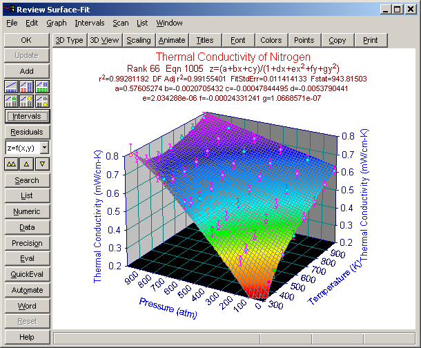
A confidence interval map is two continuous surfaces, one lower and one higher in Z values, although it must be computed at discrete X,Y values. In TableCurve 3D, this is plotted as z-bars at the data points. Confidence and prediction interval surfaces are a local measure of probability since the intervals are generally greater as the distance from the nearest point increases.

Confidence Intervals

The confidence interval gives the probability range for the true surface (as represented by this specific data).

Prediction Intervals

The prediction interval shown in the graph gives the 95% probability range for the surface that can be expected from the next identical experiment. Although they are not the same, points that lie outside a 95% prediction interval are often also outside ± 2 standard errors.

Other Surface-Fit Review Elements

Residuals

The Residuals graph is toggled on and off with the Residuals button or via the Residuals Graph item in the Window menu of the Surface-Fit graph. The Residuals window has its own menu with its own distinct graph options and output items.

If the Residuals window is not currently shown, click the Residuals button in the Surface-Fit graph.

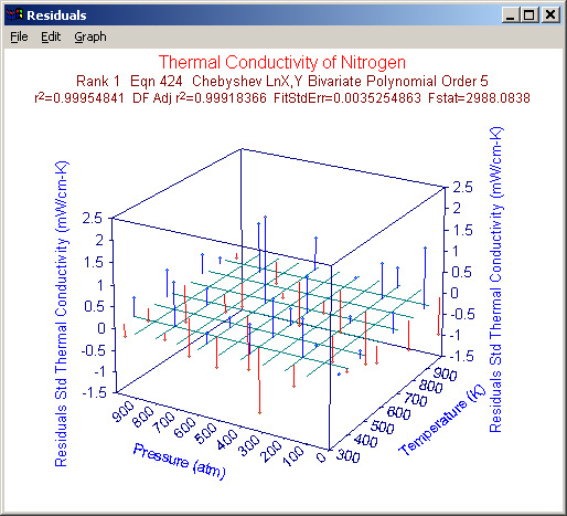
Select the Residuals Surface Graph option in the Graph menu of the Residuals Graph.

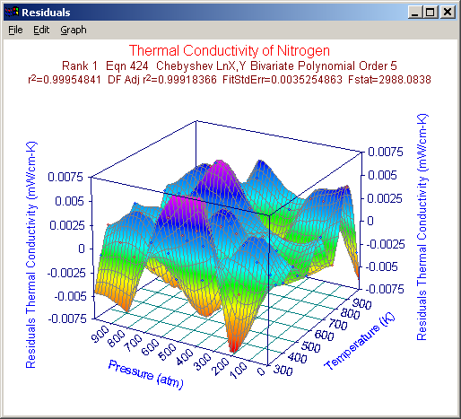
Use one of the automatic tiling options that displays the Residuals, or size and position the Residuals graph window so that the Equation List is still visible. Select a number of the initial equations and observe the differences in the residuals surface. When finished, return to the top-ranked equation.

In a residuals graph without a surface, the XY grid is drawn at Z=0 rather than at a backplane. In most instances, unfilled backplanes the best way to discern residuals when a surface is absent. A god fit produces randomly distributed residuals with no systematic trend. For some it is easier to discern systematic trends with a scatter/drop-line plot. For others, such trends are more easily observed with an interpolating surface.

Equation List Options

The Equation List window is never destroyed during the Review, but it can be hidden by toggling the List button in the Surface-Fit graph.

Toggle the Equation List off and on by clicking the List button.

Note that the Equation List has its own menu if its window is sufficiently large. If this window is very small, this menu will be absent. In this case, the List menu in the Surface-Fit graph can be used to manage most of the list-related functions, although output options will not be available. To access these output options when the equation list is too small to have a menu, maximize the list window.

There are two important concepts relative to the Equation List. One is filtering and the other is sorting. When the list is filtered, only the specified type of equation is present within the list. When the list is sorted, the contents of the current list are sorted by the specified goodness of fit criterion, floating point speed, or equation number.

To see only the simple equations, those with three coefficients, use the Equation List’s Filter menu, Choose the Simple Equations option.

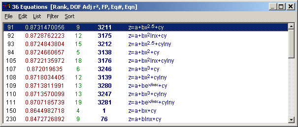
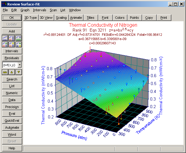
Note that none of the three parameter equations was able to produce an effective fit. Restore all equations by selecting the All Equations item in the Equation List’s Filter menu.

Note that an Arrange by Parameter Count option is available in the Sort menu to arrange the equations first by coefficient count and secondarily by goodness of fit. The value of the F-statistic sort option is covered in the Parametric Functions tutorial.

Numeric Summary

The Numeric Summary is toggled on and off with the Numeric button. It can also be activated using the Numeric Summary item in the Window menu of the Surface-Fit Graph. The Numeric Summary has its own menu with its own distinct format and output items.

If the Numeric Summary is not currently displayed, use one of the tiling options that displays the Numeric Summary or click the Numeric button to open the Numeric Summary Window. Inspect the statistical information furnished.

Rank 1 Eqn 424 Chebyshev LnX,Y Bivariate Polynomial Order 5 r2 Coef Det DF Adj r2 Fit Std Err F-value 0.9995484095 0.9991836633 0.0035254863 2988.0838015 Parm Value Std Error t-value 95.00% Confidence Limits P>|t| a 0.590336819 0.000560549 1053.141288 0.589186668 0.591486969 0.00000 b 0.081558914 0.000846635 96.33298713 0.079821762 0.083296066 0.00000 c 0.155272136 0.00109231 142.1503013 0.153030902 0.15751337 0.00000 d 0.027236565 0.000705521 38.60488977 0.025788955 0.028684174 0.00000 e -0.08991825 0.0011185 -80.391822 -0.09221322 -0.08762328 0.00000 f 0.001806688 0.000684643 2.638875558 0.000401916 0.00321146 0.01364 g -0.00156779 0.000666695 -2.35158586 -0.00293574 -0.00019985 0.02624 h 0.015818453 0.001042338 15.17593539 0.013679752 0.017957154 0.00000 i 0.000690528 0.00099807 0.69186307 -0.00135734 0.002738398 0.49493 j -0.00238253 0.000629499 -3.78480708 -0.00367416 -0.00109091 0.00078 k -1.4478e-05 0.000634861 -0.02280429 -0.0013171 0.001288149 0.98197 l -0.00223402 0.000949775 -2.35215605 -0.0041828 -0.00028524 0.02621 m -0.00325938 0.000866621 -3.76102097 -0.00503754 -0.00148122 0.00083 n 0.002421686 0.000890415 2.719727983 0.000594706 0.004248666 0.01128 o 0.001296042 0.000673256 1.925035657 -8.5365e-05 0.00267745 0.06482 p 0.000328555 0.000661467 0.496706467 -0.00102866 0.001685772 0.62342 q 2.21894e-05 0.000927175 0.023932304 -0.00188022 0.001924595 0.98108 r 0.002444723 0.000812427 3.009158574 0.000777759 0.004111686 0.00562 s -0.00199601 0.000821383 -2.43005891 -0.00368135 -0.00031067 0.02202 t -0.00155772 0.000987704 -1.57710843 -0.00358432 0.000468885 0.12642 u -0.00085831 0.001006406 -0.85284375 -0.00292328 0.001206667 0.40125 X at Fn Zmin Y at Fn Zmin Fn Zmin 348.15 0 0.2798985331 X at Fn Zmax Y at Fn Zmax Fn Zmax 348.15 1000 0.7911115556 Procedure GaussElim r2 Coef Det DF Adj r2 Fit Std Err 0.9995484095 0.9991836633 0.0035254863 Source Sum of Squares DF Mean Square F Statistic P>F Regr 0.74278108 20 0.037139054 2988.08 0.00000 Error 0.00033558445 27 1.2429054e-05 Total 0.74311667 47 Description: Thermal Conductivity of Nitrogen X Variable: Temperature (K) Xmin: 348.15 Xmax: 973.15 Xrange: 625 Xmean: 635.65 Xstd: 214.3768803 Y Variable: Pressure (atm) Ymin: 0 Ymax: 1000 Yrange: 1000 Ymean: 500 Ystd: 345.17957091 Z Variable: Thermal Conductivity (mW/cm-K) Zmin: 0.28 Zmax: 0.79 Zrange: 0.51 Zmean: 0.5933333333 Zstd: 0.1257417707

The coefficient confidence % is controlled by the value set in the Intervals menu of the Surface-Fit graph.

The use of the statistical information in the Numeric Summary is discussed in detail in the Parametric Functions tutorial.

Data Summary

The Data Summary is toggled on and off with the Data button. It can also be activated using the Data Summary item in the Window menu of the Surface-Fit Graph. This report has its own menu with its own distinct format and output items. It contains a point-by-point summary of the fitted data.

If the Data Summary is not currently displayed, use the tiling option that displays it or click the Data button to open the Data Summary Window. From the Data window’s Type menu, explore the four different formats (Residuals, Confidence Limits, Prediction Limits, All Information) available.

Rank 1 Eqn 424 Chebyshev LnX,Y Bivariate Polynomial Order 5 XYZ * X Value Y Value Z Value Z Predict 95.00% Prediction Lim Weights 1 973.15 1000 0.775 0.7754448 0.7656207 0.785269 1 2 973.15 800 0.745 0.7469011 0.7377642 0.7560381 1 3 973.15 600 0.715 0.7123276 0.7034917 0.7211634 1 4 973.15 400 0.68 0.6799711 0.6711353 0.688807 1 5 973.15 200 0.65 0.6483551 0.6392181 0.657492 1 6 973.15 0 0.62 0.6231541 0.61333 0.6329783 1 7 873.15 1000 0.75 0.7495822 0.7408681 0.7582963 1 8 873.15 800 0.72 0.7158817 0.7074065 0.7243569 1

Inactive points are displayed in the Data Summary, but are grayed out.

When printing a data summary with All Information, use landscape mode or a very small font size.

The confidence % for the Review is a global item set in the Intervals menu of the Surface-Fit graph.

Precision Summary

The Precision Summary is toggled on and off with the Precision button. It can also be activated using the Precision Summary item in the Window menu of the Surface-Fit Graph. The Precision Summary also has its own menu with its own distinct format and output items.

The first section measures the average, minimum, and maximum absolute error at the eight points nearest the boundaries of the data and at the point closest the center of the data region when successively fewer digits of precision are used within the coefficients.

The second section measures these same errors when linear coefficients are removed or zeroed one at a time.

Click the Precision button to open the Precision Summary window. Size and position the window and inspect the information furnished. When finished, either close the Window directly, or click the Precision button, if visible.

Rank 1 Eqn 424 Chebyshev LnX,Y Bivariate Polynomial Order 5

Precision Avg Abs Error Min Abs Error Max Abs Error 18 5.333873e-19 2.609793e-19 8.40289e-19 17 7.624798e-18 1.652869e-18 1.195434e-17 16 1.31063e-17 4.404229e-18 5.616654e-17 15 7.741567e-16 2.635547e-17 2.576785e-15 14 6.153016e-15 2.851721e-15 8.981223e-15 13 4.801085e-14 7.082183e-15 1.019509e-13 12 5.067401e-13 2.99937e-14 1.674336e-12 11 2.907063e-12 6.799036e-13 6.461785e-12 10 7.867414e-11 6.665509e-12 2.702385e-10 9 6.911663e-10 9.689656e-11 2.272254e-09 8 4.837267e-09 1.517898e-09 7.482709e-09 7 5.057632e-08 2.234388e-08 8.8736e-08 6 4.100904e-07 2.963807e-08 1.336272e-06 5 6.925349e-06 8.410348e-07 2.261505e-05 4 7.526112e-05 4.102642e-06 0.0002286653 3 0.0005189072 8.004486e-05 0.000899817 2 0.0064797038 0.0001352422 0.0210595354 Removing Avg Abs Error Min Abs Error Max Abs Error a 1.0706991763 0.7462118516 2.1091100844 b 0.1079785039 0.0196921938 0.2913874286 c 0.1952497744 0 0.5547443734 d 0.0484539669 0.0344282223 0.0973087077 e 0.0833796682 0 0.3212530157 f 0.003276807 0.0022837341 0.0064547978 g 0.0023745512 0.0010911641 0.0056012829 h 0.0195211088 0 0.0565149553 i 0.0009142121 0.0001667262 0.0024670643 j 0.0029959608 0 0.0085121348 k 2.430731e-05 1.57501e-05 5.172428e-05 l 0.0023587035 0 0.0079815317 m 0.0057984534 0.004120002 0.0116448671 n 0.0022455881 0 0.0086520126 o 0.0023506437 0.0016382549 0.0046304008 p 0.0005489998 0.0003511581 0.0011738352 q 2.588686e-05 0 7.927667e-05 r 0.003702738 0.0017014982 0.0087343171 s 0.0024632173 0 0.0071311837 t 0.0020623122 0.0003761068 0.0055652916 u 0.0010792936 0 0.003066493

Evaluation

The Evaluation feature is a powerful means for extensively evaluating the equation or equations under consideration as approximating functions. The Evaluation is opened with the Eval button. It can also be opened using the Evaluation item in the Window menu of the Surface-Fit Graph.

Click Eval to open the Evaluation window. Enter 500, 500, 0.6, 800 and 800 in the five fields and then click each of the calculation types. Note the computation of a function value, roots, derivatives, and volume.

Click the Automatically Generate Table Entries option. Be sure that Generate, To Evaluation Table, and X and Y Inout, Z=Fn at X,Y are selected and click OK. Accept the X and Y grid by clicking OK.

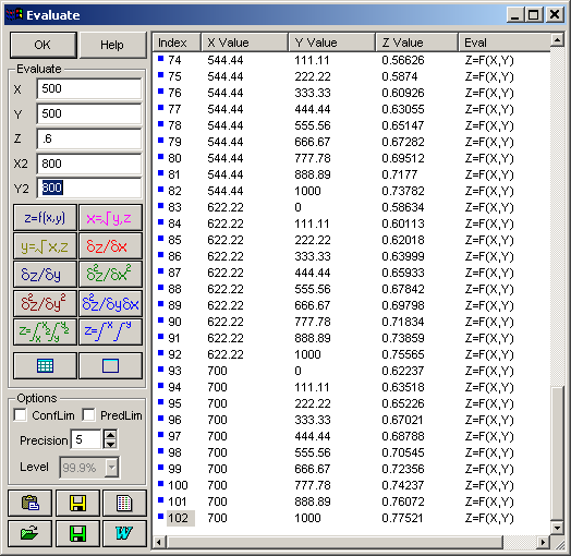
The Generate Table feature is a powerful means for generating data based upon the current surface-fit equation. The X,Y values can be generated or read from file and written either to the evaluation table or directly to a file.

Click OK to close the evaluation.

Surface Fit Output Options

Export and Output Options

Each of the key Review windows has its own output. If it is a text or equation list window, the contents can be saved to an ASCII, WK1, RTF, or MS Word file, copied to the Windows clipboard, or printed.

The Residuals Graph window offers a printed graph, clipboard or file metafiles, clipboard bitmaps, as well as an ASCII or WK1 file of the numeric values of the residuals.

The Surface-Fit Graph window offers a printed graph, including a half-page graph with half-page numeric summary. The graph can be saved as a file-based metafile or it can be copied to the clipboard as either a metafile or bitmap.

The Surface-Fit graph’s File menu also includes the following frequently used export options:

• Excel XLS spreadsheet file with four possible formats. All include a generated data section
• SigmaPlot notebook file with four possible formats
• Code Generation in C, PASCAL, FORTRAN 77, FORTRAN 90, BASIC, Matlab, C++ and Java languages
• ASCII output of generated data with three possible formats
• ASCII output of parameters to full precision with optional identifiers
• ASCII output of covariance matrix

Printed Graphs

To see the quality of a TableCurve 3D printed graph, click the Print button above the Surface-Fit graph. Choose the format and options desired and press OK to initiate the print.

Metafiles and Bitmaps

To paste TableCurve 3D graphs into other programs, such as to an Excel file containing the original data, copy the graphs as bitmaps or metafiles to the clipboard. File export options include Aldus format metafiles and device-independent bitmaps.

Click the Copy button in the control panel of the Surface-Fit graph. Choose the format and options desired and press OK.

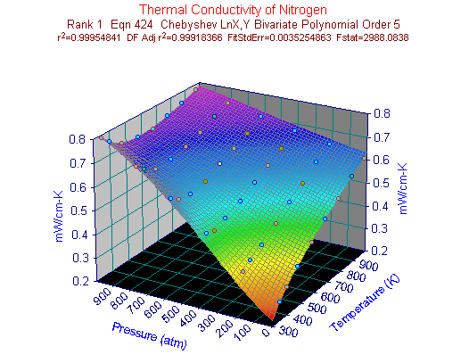
Excel

To see the Excel export capability, select the Save Excel option in the Surface-Fit graph’s File menu. After selecting the format, press OK to proceed. Enter any file name.

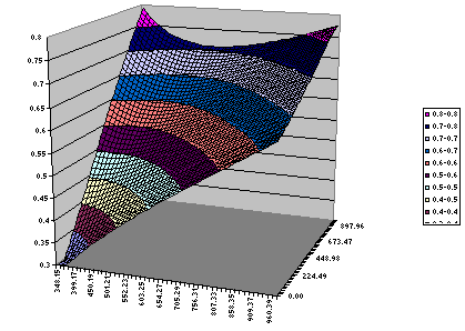
Note that the initial values in the generated value fields duplicate the vertices in the TableCurve 3D Surface-Fit graph.

The Full Worksheet option writes an extensive spreadsheet file containing equation and parameter information, raw data information, and a full generated section. Other options write only the Generated Information, or basic XYZ files in a column format, or in the matrix format that Excel requires in order to plot a 3D surface.

SigmaPlot

For SigmaPlot users, select the Save SigmaPlot option in the Surface-Fit graph’s File menu. Select the SP2000/2002/ format and accept the generated data defaults. Click OK to proceed. Enter any file name.

Language Code

For those involved with scientific programming, the code generation capabilities of TableCurve 3D represent a strong analytical asset.

Select the File Menu’s Code Generation option and then select the Full Test Code option and the program language of choice. Specify the function, subroutine, or procedure name for the function code containing the fitted equation. Press OK and then input a file name. The correct language extension will be appended. The code is then generated and an ASCII listing of the file follows as a confirmation. Inspect the generated code and then close the list window.

The generated code is written to a full 15-16 or 18-19 digit precision. Code can be generated for all of TableCurve 3D’s 453,697,470 equations. Except for Matlab where it is not needed, the full test code will include a simple calling routine to test function evaluations. If the equation contains the error function or a series evaluation, its code is also automatically generated.

Click the OK button in the Surface-Fit graph to exit the Review and return to the main program window.

Surface Fit Output Items

TableCurve 3D stores the necessary information to recreate all of the fits available in the Review, but does not save the results of all of the fits. When the main window graph is clicked, and it reflects a surface fit, the equations previously fitted are again fitted using the same preferences previously applied.

Select the first of the six surface fit items and click in the center the main graph window.

This places the Review in the state it was in when this surface fit item was previously added to the TableCurve 3D notebook. The same equations are available in the Equation List and the equation comprising the surface fit object will be selected. Any graph customizations previously made are also restored.

Click the OK button in the Surface-Fit graph to once again exit the Review and return to the main program window.

Annotation Items

These items are useful for adding experimental notes to a TableCurve 3D notebook file. An annotation item can only be added to an XYZ data node.

Select (left-click) an XYZ data item in the notebook hierarchy and then right click the item to open the popup menu. Select Annotate. Enter a few words or lines into the editor that overlays the statistics window. Close the Annotation window.

When an annotation item is selected, its text is displayed in the statistics window. Since the ASCII editor can open any ASCII file, the content of such files can be easily added to the TableCurve 3D notebook file.

Exiting TableCurve 3D

To exit TableCurve 3D, either close the main TableCurve 3D window, or use the Exit item in the main File menu.

The second tutorial covers parametric functions and focuses on TableCurve 3D’s non-linear equations and user-defined functions.