Prediction and Forecasting
This tutorial covers the prediction capabilities of TableCurve Studio.
A prediction procedure applies to data with equally spaced x-values and generates estimates additional discrete x values, at one or both ends of a data stream, as in time-series forecasting. No interpolation occurs and there is no continuous function, although it is possible to estimate or predict an arbitrary number of additional data values with this same x-spacing.
An estimation procedure, on the other hand, is one where the set of x values used for the computation of y values is arbitrary and user-defined. Interpolation is always possible, and as with curve-fit equations, extrapolation or prediction is available, though not always wise. A continuous function, or the means to simulate such, is the central feature of the procedure.
TableCurve Studio offers a single prediction procedure based upon autoregressive modeling.
AR Linear Prediction
An AR (Autoregressive) model forecasts future values by a linear relationship with some number of prior values. It can also be used to back forecast prior values by a linear relationship with some number of subsequent values. In this example, we will only explore the prediction of future values.
Start TableCurve Studio. Select Start/Programs/TableCurve Studio v5.
 Select the File menu’s Import option (or use the Import button in the main toolbar). If Excel [xls] files are not shown, click on the Files of Type drop-down button and select Excel [xls] files. Select and open the file SAMPLE.XLS.
Select the column with the label (10)Prediction!I: Prediction 6dB Time to be used as the X-variable in the data table. Select the next column identified in the selection list as (10)Prediction!J: SN6dB for the Y-variable. Check Import Preview to see a graph of the data that will be imported.
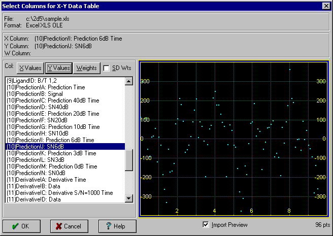
Note that the first two selections are automatically placed in the X and Y positions. You may double click on the column for the Y variable in order to immediately proceed with the read operation. You can also revise the initial X,Y selections as well as to specify a column to be used for the weights. The weights can be optionally imported as standard deviations.
Press OK to accept these choices. Press OK once again within the titles dialog to confirm the imported titles.
This data set consists of the sum of three different sinusoids and 50% Gaussian noise.
Autoregressive Fitting
 Select the AR Modeling and Prediction option in the Estimate menu or Process toolbar.
Select the Data Fwd algorithm, be sure Single Order is checked, and that the order is set to 40. Be sure Stabilization is set to None. Set the Predicted Points n to 48.
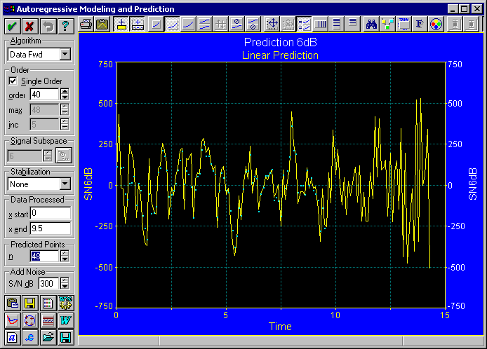
The Data Fwd algorithm is really one of the best AR methods for prediction since it performs a least-squares minimization when it computes the coefficients. The AR procedures in many software packages employ reflection coefficient or autocorrelation based algorithms which produce results that are even less credible.
Still, it would not be much of a reach to assume that this prediction is nonsense. But is it?
Ascertaining Nonsense
This is one of the most important elements in using AR Prediction wisely. One of the best ways to assess the validity of a prediction is to see if the same trends are found at a variety of model orders. TableCurve Studio makes this easy.
Uncheck Single Order. Enter 10 for min, 40 for max, and 5 for inc. Zoom in on only the predicted portion of the graph.
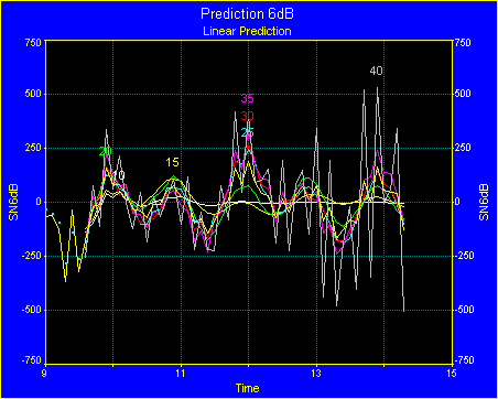
There is an indication of common upward and downward trends at certain values of time, suggesting some validity to the prediction. It is well known, however, that AR predictions are very sensitive to model order. So much is this expected with traditional AR modeling that an extensive measure of research has gone into developing various numeric criteria for identifying the optimum model order.
 Click on Plot Selection Criteria.
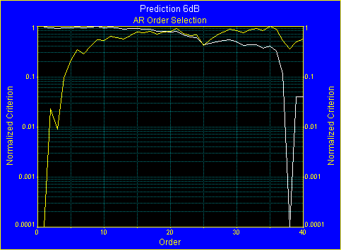
The white curve is a normalized AIC (Akaike Information Criterion) and the yellow curve is a normalized MDL (Minimum Description Length). The minimum in these criteria are possible optimum model orders. Both criteria suggest 38 as the optimum model order.
Check Single Order. Enter 38 for the order. Right click in the graph area to restore standard scaling.
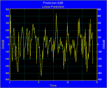
The order 38 prediction does appear slightly more stable. One of the best ways to check for validity with any given AR fit is to use only a portion of the data series to compute the AR model and use the remainder as a check for accuracy in the prediction.
In the Data Processed box, enter 7.8 for x end and set the Predicted Points n to 17. Zoom in on the predicted region.
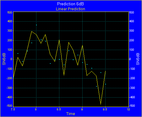
It is hard to argue with what is evident here. The prediction does roughly track the data. In this case, the prediction cannot be dismissed as nonsense.
Assessing Stability
A set of AR coefficients is a filter that is applied to the end of the data to generate the future values. It is important to verify that the coefficients are stable. The complex roots of an AR polynomial must fall on or within the unit circle in order to have a stable filter.
 Click the Plot Roots button.
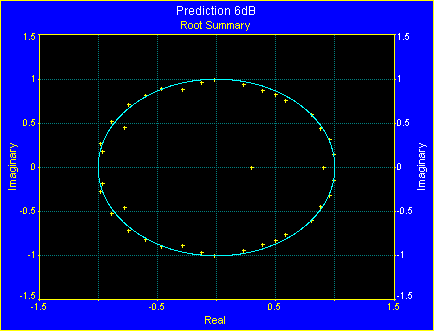
Unlike the autocorrelation and reflection coefficient AR algorithms, a least-squares minimization does not insure that these complex roots will be in or on the unit circle. Here they are close, but note the warning that 14 of these roots are outside the unit circle.
Check the Magnitude box.
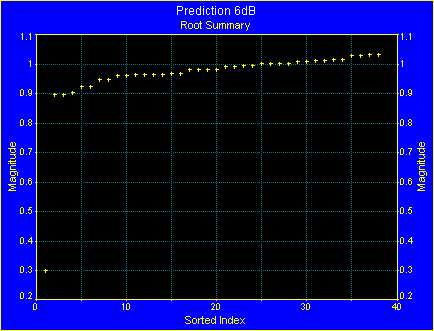
The roots with a magnitude greater than 1.0 are outside the unit circle. Here it is evident that a significant number of roots are outside and contributing to an instability in AR predictions.
In harmonic analysis, the inspection of complex roots can help identify the number of harmonics present. Roots very near the unit circle are typically associated with signal harmonics and those in the interior are generally attributable to noise. This data set was generated by summing three sinusoids and adding a large measure of noise. There should thus be six roots very close to the unit circle and the remainder should be in the interior. Clearly that is not evident here.
Stabilizing an AR Fit
The set of AR coefficients can be stabilized in one of two ways. The roots can be reflected back into the interior of the unit circle. This is the choice to make if the roots most removed from the unit circle represent noise. They can also be mapped directly to the unit circle. This is the option to use if these roots furthest from the unit circle represent harmonics. The easiest approach is to try both stabilizations and see which is most effective.
 Click OK to close the Complex Roots plot. For the Stabilization, select Reflect Out.
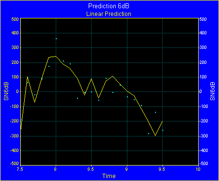
There is a lot to like about this stabilization which assumes the outlier roots are due to noise.
For the Stabilization, select Unit Circle Out.
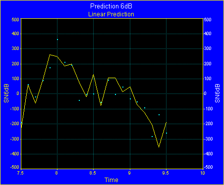
Reflecting the outlier roots to the unit circle, assuming they represent harmonics, also results in an improved prediction.
SVD Autoregressive Prediction
While we appear to have a respectable prediction, can we do better? Indeed, we can. It is possible to compute the AR coefficients using SVD (singular value decomposition) to remove the influence of noise on the AR coefficients. In this case, the model order is far less important, since most of the eigenmodes are going to be discarded anyway.
It is important to fit a high enough model order to manage the noise that is present, and it is crucial that a signal space be selected. Unlike the optimum model order identification for traditional AR fitting, which is often tricky, signal space identification is often straightforward.
Right click in the graph area to restore standard scaling. Select the Data Svd Fwd algorithm. Leave the order at 38 and set the Signal Subspace to 2. Set the Stabilization to None. Set x end to 9.5 and set the Predicted n points to 48.
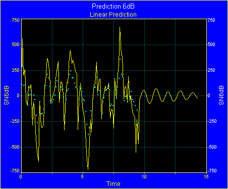
A signal space of 2 accommodates only a single harmonic. We know that this data set was constructed from three sinusoids and that the correct signal space should be 6.
Click on the Graphically Select Signal and Noise Sub-Spaces button. Click on the 6th eigenmode.
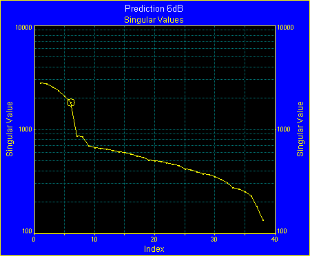
A singular value plot is often sufficient for setting the signal space. This is the eigenmode count used for computing the AR coefficients. Ideally, this plot will reveal a transition to a long sloping noise floor. The last eigenmode representing signal space should be just prior to this transition.
In this plot there are two possible signal spaces, 6 and 8. We will explore each.
Click OK to update the signal space to 6.
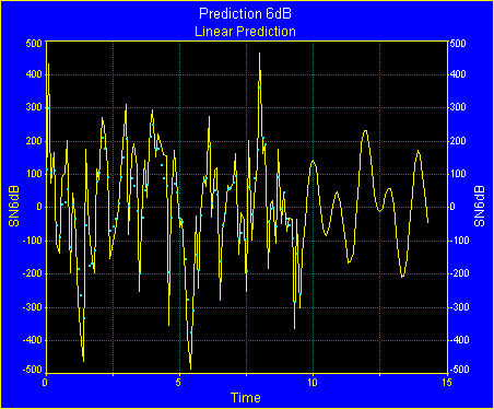
Change the signal space to 8 and then back to 6. Note that there are only minor differences in the prediction. The prediction is certainly smooth, but predictions using the SVD algorithms will usually be smooth. The same questions that were applicable to traditional AR prediction also apply to SVD-based algorithms.
Uncheck Single Order. Enter 10 for min, 40 for max, and 5 for inc. Zoom in on only the predicted portion of the graph.
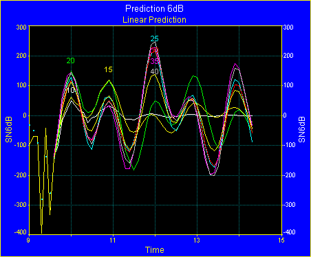
The model orders 25, 30, 35, and 40 are all very close.
Check Single Order. Enter 40 for the order. Right click in the graph area to restore standard scaling. In the Data Processed box, enter 7.8 for x end and set the Predicted Points n to 17. Zoom in on the predicted region.
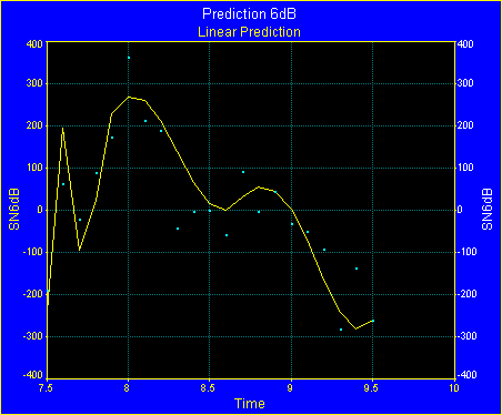
The predicted curve looks almost like a smoothed data sequence.
Click the Plot Roots button.
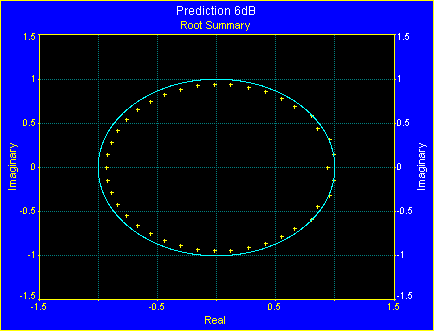
Only 2 roots are outside the unit circle now. Six are very near the unit circle and the remainder are in the interior.
Check the Magnitude box.
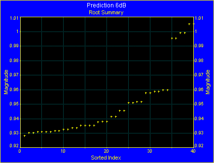
Now we have the three harmonics centered about the unit circle and the roots associated with noise well toward the interior. Whether the two outlier roots are reflected into interior of the unit circle or mapped to the unit circle proper, they will still be very close to the other two harmonics. Since this profile offers a clear indication these roots are associated with harmonics, we will map these roots to the unit circle.
Click OK to close the Complex Roots plot. For the Stabilization, select Unit Circle Out.
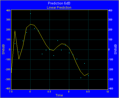
The stabilization produced only minor changes.
Influence of Noise
A prediction model should be stable under the influence of added white (Gaussian) noise.
Set the S/N dB to 6.
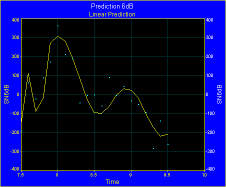
This adds another 50% random Gaussian noise to the data on top of the 50% noise originally present. Note that the plotted data remains the original. The AR coefficients, however, are now computed based on the data with this specified amount of added noise. The AR filter is still offering very good predictions, despite this large measure of added noise.
Set the S/N dB back to 300, the floating point double precision significance limit where no noise is added. Right click in the graph area to restore standard scaling. Set x end to 9.5 to process the full data series.
 Click on the View Residuals button.
 In the Residuals window, click on Display Basic Residuals.
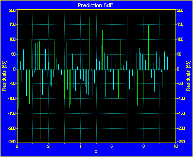
The AR model order fit should produce residuals that are comparable to a good parametric fit. That is, there should be no systematic trends in the residuals and they should be normally distributed.
In the Residuals window, click on Display Residuals in Stabilized Normal Probability Plot.
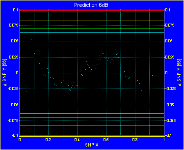
Here the residuals show no apparent systematic trend and are easily judged normally distributed.
Fit Statistics
Fit statistics are also reported. Note that the r² is 0.73, very high for a data set with 50% random noise added.
Not all data can be predicted from a linear combination of previous values. Truly stochastic data (all noise and no deterministic signal) will have very poor AR fit statistics.
To preserve the current settings, click OK to close the AR Modeling procedure. Answer No to updating the data table.
 Select the Generate Data option in the Edit menu or main toolbar. Enter Y=IF(X==0,1,0) as the data function. Set the Gaussian Noise % to 1000. Be sure X goes from 0 to 1 with a 0.01 increment. Click OK.
Click OK to accept the generated data and answer Yes to update the data table. Click OK to accept the titles.
Return to the AR Modeling and Prediction option.
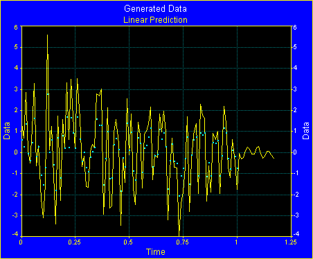
This particular white noise data set has an r² value of 0.011. The value you see will be different, but it should be very low. An AR fit is no different from a parametric one. Unless you have strong fit statistics, the model is not valid.
 Click on Cancel to exit the procedure. Exit the program by closing the main window or by the Exit item in the File menu.
Predictions in the Real World
The AR prediction algorithm is useful for processing data containing significant deterministic components. Data that are indistinguishable from noise will not be predicted successfully. Even when deterministic components are present, they may be too complex to be modeled by a linear combination of previous values.
TableCurve Studio's prediction procedure offers robust effective algorithms that can manage a large measure of observation noise. The key to valid predictions using them rests almost entirely on whether a successful fit to the underlying data trend can be realized. Some data sets will be favorably described by an AR model and others will not.