Derivative Estimation

In this tutorial, we will explore the different procedures TableCurve Studio offers for generating accurate estimates for derivatives.

Approaches

There are five ways to estimate derivatives in TableCurve Studio:

• • Fit a parametric model and generate analytic or numeric first and/or second derivative estimates. For a parametric model, noise is not a factor. The derivatives are computed from the curve-fit equation. If the default analytic derivatives are set, the generated derivatives will contain full numeric precision. Accuracy, however is a different matter. The derivatives will only be as accurate as the model selected to fit the data.
• • Fit a non-parametric smoothing spline to the data and evaluate the analytic derivatives of the spline. A spline's derivatives are strongly influenced by noise. If any noise at all is present within a data stream, some form of smoothing will be needed. As with least-squares parametric fitting, the spline coefficients for a smoothing spline are computed in an overspecified sense. The number of knots (nodes where segments meet) in the spline will be fewer than the number of data values.
• • Fit an interpolating spline to data that have been pre-smoothed and compute the derivative analytically from the spline. In this instance, the number of nodes in the spline will be equal to the data count. For this approach to work effectively, a very high level of smoothing is required.
• • Perform a Fourier decomposition of data and compute derivatives from the individual sine components. Fourier interpolation is slow and highly sensitive to noise. A Fourier procedure must be combined with a lowpass filter in the frequency domain in order to produce reasonable derivative estimates.
• • Locally fit polynomials with a sliding window across the data and directly create a derivative filter of the desired order. A Savitzky-Golay derivative filter is usually the most accurate non-parametric approach for estimating derivatives. It is also the only recommended approach for derivatives beyond second order.

Importing A Noisy Sinusoid Data Set

Start TableCurve Studio. Select Start/Programs/TableCurve Studio v5.

Select the File menu’s Import option (or use the Import button in the main toolbar). If Excel [xls] files are not shown, click on the Files of Type drop-down button and select Excel [xls] files. Select and open the file SAMPLE.XLS.

Select the third column with the label (11)Derivative!E: Derivative S/N=100 Time to be used as the X-variable in the data table. Select the fourth column identified in the selection list as (11)Derivative!F: Data for the Y-variable.

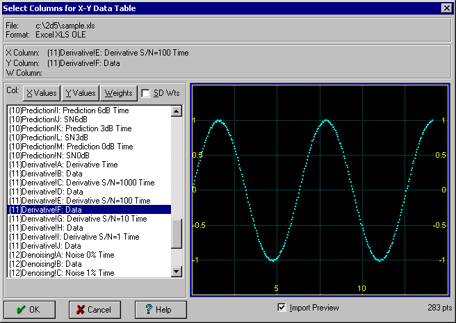
Press OK to accept these choices. Press OK once again within the titles dialog to confirm the imported titles.

This sinusoid contains 1% added Gaussian noise. This may sound very small, but it is enough to render most derivative estimation algorithms useless, especially for derivatives beyond first order. The data are scaled so that the second derivative should be a cosine wave rather than a sine wave, and equal in both magnitude and phase. Also, the fourth derivative should exactly overlay the original sine wave. This is the classic test case for evaluating the accuracy of derivative algorithms.

Fitting a Parametric Model

Click the Curve Fit Waveform Functions option in the Process menu or toolbar.

When the fit is concluded, enter the Review by clicking the Graph Start button.

As an alternative, you may press OK and select the Graph Start item in the Review menu. If you do not respond to the conclusion of the fit in 10 seconds, the Review is automatically started.

In the Equation List, select Equation 8014, the sine wave model.

Click the Set Y2 Axis Content button and select Curve-Fit,Data in Y1; First,Second Derivatives in Y2. Click OK.

Select the Preferences option in the File menu of the Curve-Fit graph. Be sure the Analytic Curve-Fit Equation Derivatives is checked. Click OK.

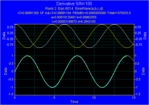
This sine wave data set was generated with a zero mean, an amplitude of 1.0, a phase of 0, and a wavelength of 2p. Note that the parameters are recovered to about four decimal places. The white curve in the Y2 plot is the first derivative and the yellow curve is the second derivative. Note that the second derivative is identical to the data except for the sign.

Derivatives are generated:

In the Excel, Lotus, and SigmaPlot export options

In the Copy procedure of the Curve-Fit graph

As one of the Generate Table options in the Evaluation procedure

To test the accuracy of the second derivative, we will copy the curve-fit information to the clipboard. Second derivative evaluations are automatically included.

Click the Copy button in the control panel of the Curve-Fit graph.

Click the Set Y2 Axis Content button and select Curve-Fit,Data in Y1. Click OK.

Click OK to close the Review.

To make this data more convenient for repeated import, we will save it as an SPSS file. This data can then be reimported in one step by selecting the file from most recently used list in the File menu.

Click the Save As button in the main toolbar. Set the Save As Type to SPSS [sav] and enter tour4. Clock OK.

Select the Import Clipboard button or File menu item. Select Column K: X Observed for the X variable and Column U: Second Deriv for the Y variable. Click OK to initiate the import. Click OK to accept the titles.

We will now employ a little trick to fit this second derivative data to the expected underlying parametric function, the second derivative of the sine function with an amplitude of 1.0, a phase of 0.0, and a wavelength of 2p.

Select the User Functions option in the Process menu or toolbar. Enter d2sine for the name, enter 1 for the parameter count, enter Y=A0*0-SIN(X) as the function expression. Click OK to exit the UDF procedure and reply OK to the message that indicates A0 was found to be insignificant.

Select the Curve-Fit User Functions option in the Process menu or toolbar. When the fit is concluded, enter the Review by clicking the Graph Start button.

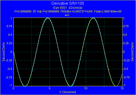
Since none of the parameters are adjusted in the non-linear fit, we compute a correlation with the underlying second derivative function. The standard error is 0.00074. Thus a non-linear least-squares sine fit generates an analytical second derivative accurate to this measure.

We will now generate second derivative data sets using each of the other four approaches for estimating derivatives. We will then similarly assess the accuracy of these estimations.

Click OK to close the Review.

Non-Parametric Smoothing Spline

In this approach, we will fit a smoothing spline to the data and evaluate the analytic derivatives of the spline.

Select tour4.sav from the first position of the most recently used files list in the File menu. Answer No to save the existing data and click OK to accept the titles.

Select the Spline Estimation option in the Process toolbar or Estimate menu.

Select the Cubic procedure, set Output Data to 1st Deriv, and set n to 283 to exactly match the incoming data.

By default, the n is set to perform a 2x upsampling.

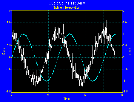
Even at a 1% noise level, the first derivative of an interpolating spline is barely stable.

Set Output Data to 2nd Deriv.

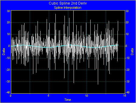
All accuracy is lost.

Select the Cubic smooth procedure. Set Output Data to 1st Deriv.

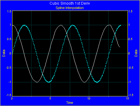
This "cross-validation" smoothing spline is probably the most widely used of all smoothing splines. A cubic (order 3) spline produces smooth first derivatives and continuous (but not smooth) second derivatives.

Set Output Data to 2nd Deriv.

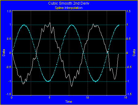
Since most users want both continuity and smoothness, the Cubic Smooth procedure is generally only of value for first derivatives. To get smooth second derivatives, a quartic (order 4) spline is needed.

Select the LS B-Spline fix procedure. Set the Order to 4 and the Knots to 12.

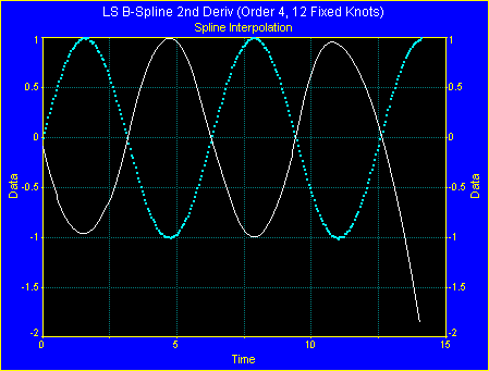
The shape is irregular because the knots are not placed at the crests, troughs, and inflection points. There are two options, a non-linear optimization that seeks to find these optimum knots, and a direct specification of them.

Select the LS B-Spline opt procedure.

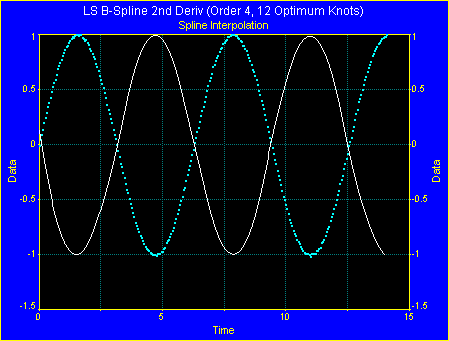
Click OK to close the estimation procedure and answer Yes to updating the data table.

Select the Curve-Fit User Functions option in the Process menu or toolbar. When the fit is concluded, enter the Review by clicking the Graph Start button.

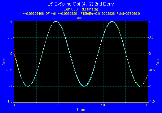
The second derivative's standard error relative to the underlying generating function is 0.0192.

Click OK to close the Review.

Click Reset XY Data to restore the original sinusoidal data with the 1% noise.

Fitting an Interpolating Spline to Pre-smoothed Data

Select the Smoothed Data Spline Estimation option in the Estimate menu or Process toolbar.

Select the Eigendecomp. procedure, set the B-spline order to 4, set output data to 2nd Deriv, and set n to 283.

Click the AI Expert button.

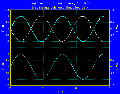
In all cases, including Savitzky-Golay, this procedure smoothes the raw data, a B-spline is fitted to the smoothed data, and analytic derivatives are computed from the B-spline interpolant. Note that the zero order smoothing in the lower plot looks good for most of the algorithms. The analytic second derivatives in the upper plot are not going to win many awards, although the Eigendecomp. procedure is probably the most accurate.

Click OK to close the estimation procedure and answer Yes to updating the data table.

Select the Curve-Fit User Functions option in the Process menu or toolbar. When the fit is concluded, enter the Review by clicking the Graph Start button.

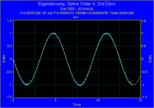
The second derivative's standard error relative to the underlying generating function is 0.0588.

Click OK to close the Review.

Click Reset XY Data to restore the original sinusoidal data with the 1% noise.

Fourier Derivative Estimation

Select the Fourier Estimation option in the Estimate menu or Process toolbar.

Select the cs3 BHarris 3 window, enter 0.3 for Freq1. and set the Output Data to 2nd Deriv.

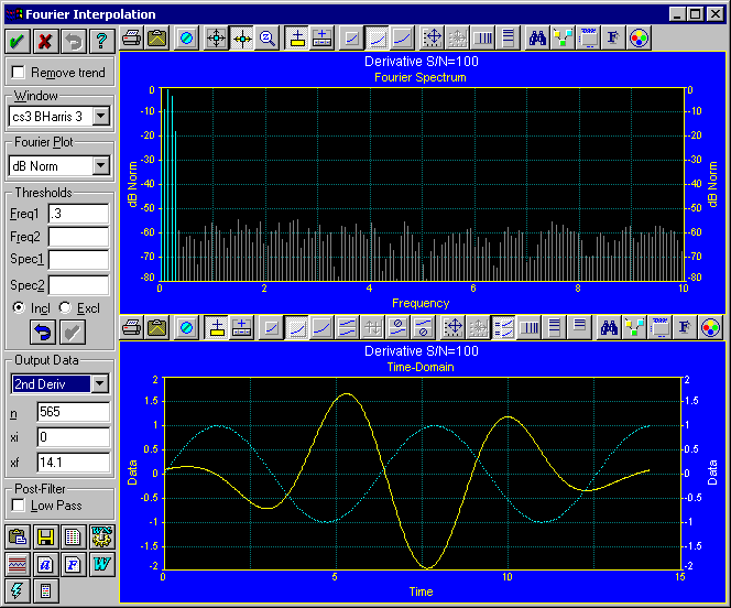
Note that a data taper is needed to isolate the harmonic and filter the noise. The second derivative is smooth and hints at the true shape, but accuracy is very poor.

Click Cancel to exit the Fourier Estimation procedure.

Savitzky-Golay Derivative Filters

Select the Savitzky-Golay Spline Estimation option in the Estimate menu or Process toolbar.

This option creates a filter that smoothes directly to the derivative order of choice. A constrained cubic spline is then fit to the derivative data in order to provide continuous estimates. This procedure was designed for accuracy in derivatives.

Set the one-sided sliding window (Win n) to 32, be sure the order is 4, and set Passes to 1. Check the Zero Edges box. Set Process to 2nd Deriv and set n to 283, the size of the incoming data.

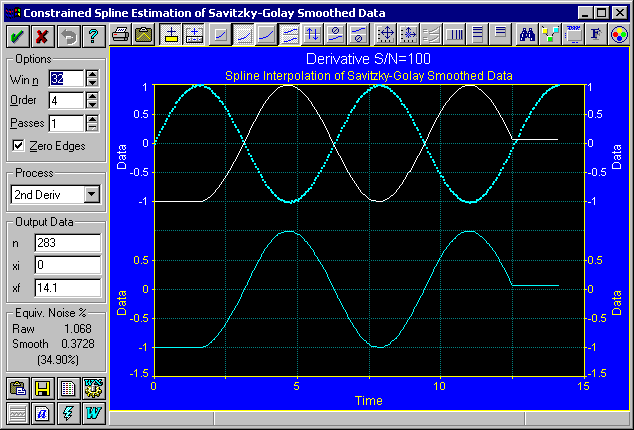
The Zero Edges option treats edge effects in the filter by holding the estimate constant at the last value where edge effects are absent. In general, a properly designed Savitzky-Golay derivative filter will be very accurate except in these edge effect regions. We will now change the exported range so that these edge effect regions are excluded.

Set xi to 1.8 and xf to 12.5.

Click OK to close the estimation procedure and answer Yes to updating the data table.

Select the Curve-Fit User Functions option in the Process menu or toolbar. When the fit is concluded, enter the Review by clicking the Graph Start button.

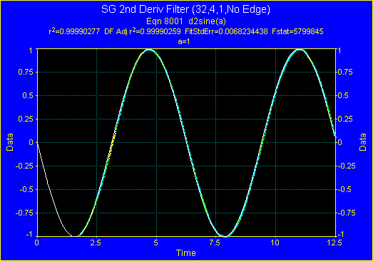
The second derivative's standard error relative to the underlying generating function is 0.0068. This is an excellent accuracy.

Click OK to close the Review.

Click Reset XY Data to restore the original sinusoidal data with the 1% noise.

Again select the Savitzky-Golay Spline Estimation option in the Estimate menu or Process toolbar.

Set the one-sided sliding window (Win n) to 54, set the order is 6, and be sure Passes is set to 1 and the Zero Edges box is checked. Set Process to 4th Deriv.

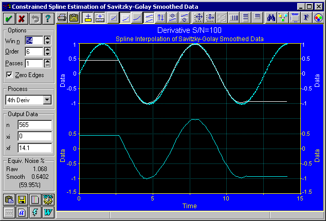
Although you will generally need to remove the edge effect regions and go to higher window sizes, it is possible with this procedure to get accurate higher order derivatives. The fourth derivative of a scaled sine wave is the original function. Very few derivative algorithms are capable of accurately resolving a fourth derivative.

Set the one-sided sliding window (Win n) to 100, set the order is 10, and be sure Passes is set to 1 and the Zero Edges box is checked. Set Process to 8th Deriv.

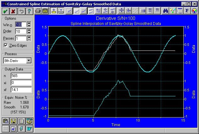
Like the fourth derivative, the eighth derivative of a scaled sine wave will be the original waveform. Given the size of the data set, the zone free of filter edge effects is small. Still, the eighth derivative is valid and has reasonable accuracy.

For accurate higher order derivatives, this Savitzky-Golay Spline Estimation option is algorithm of choice.

Since we are not interested in updating the data table, click on Cancel to exit the procedure.

Exit the program by closing the main window or by the Exit item in the File menu.