Least Squares Curve-Fitting
Linear Equations
A linear equation is one whose coefficients appear linearly in the expression. For example, the following equation is linear in its coefficients:

Here the coefficients a, b, c, and d linearly multiply the 1, x, x^2, x^3 basis functions of x. Such linear equations can be solved in a single step matrix solution.
Note that linear equations refer to the relationship between the coefficients and basis functions, not to the graphical appearance of the curve. A curve may have a wildly non-linear appearance, but yet be formed by a linear equation.
Non-Linear Equations
A non-linear equation, on the other hand, is one where the coefficients appear in a non-linear or nested fashion. The following equation is linear only in the a and b coefficients, and non-linear in c and d:
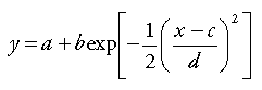
A non-linear equation cannot be solved in a single step. Estimates must be made for each coefficient, and some form of iterative convergence must follow.
Minimization of Least Squares
In TableCurve 2D, the fitting of linear equations always minimizes the sum of squares of the residuals. A residual is defined as:

A residual is simply the difference between the y value of a given x,y data pair and the y value computed from the curve-fit equation at this same x value. A residual is thus the vertical y-distance between the curve and a data point. It can be either positive or negative in value. The square of a residual is always positive, and thus reflects the magnitude of the residual, although it does so in a second order rather than a linear fashion.
Least squares minimization thus assumes that the x values are accurately determined, and that an error exists only in the dependent variable y. In doing a least squares minimization, one assumes that the errors map to a Gaussian profile. Such errors are said to be normally distributed.
Design Matrix
In a linear equation it is possible to construct a design matrix based upon the sums of the basis functions and their cross-products. Let us consider the simple equation for a quadratic:

The first step is to construct the least squares merit function. This is often referenced as the chi-square:

This is simply the weighted sum of squared residuals. The goal of all least squares curve-fitting is to minimize this chi-squared function. To do this, we must take its partial derivatives with respect to each of the parameters:
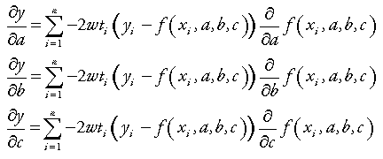
The chi-squared will be at a minimum when these three partial derivatives are zero. By setting these three equations to zero and taking the partial derivatives of this quadratic equation, the following design matrix and constant vector is produced:
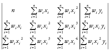
Note that the weights wi are inverse variances or 1/si^2, where si is the standard deviation for a given data pair. TableCurve 2D assumes wi‘s of 1.0 unless specific weights are entered.
The determination of a, b, and c requires no more than the computation of a handful of sums and the solution of the three simultaneous equations, a very fast procedure compared to the iterative procedure required for non-linear equations.
Non-Linear Least Squares Fitting
When an equation is non-linear, the least squares procedure is similar. In this instance, however, it is not possible to express partial derivatives as a function of only the x basis functions. In a non-linear equation, the partial derivative with respect to one coefficient will include one or more of the other coefficients, making a single step matrix solution for the individual coefficients impossible.
As such, non-linear fitting consists of an iterative procedure that begins with an initial set of estimates for the parameters. Although there are a variety of methods to converge to the minimum least squares solution, all procedures must compute a point by point sum of squared residuals for each iteration’s set of coefficients. This is especially time consuming with large data sets.
TableCurve 2D uses the Levenburg-Marquardt algorithm for fitting its non-linear equations and user-defined functions. Although this algorithm requires a matrix inversion and the computation of partial derivatives for each iteration, its rate of convergence is among the best of available methods.
Global vs. Local Minimum
Unlike linear fitting, non-linear fitting does not guarantee the minimum least squares solution. Non-linear fitting algorithms sometimes find a local minimum in the n-dimensional space of the fit rather than the true global minimum which represents the desired least squares solution. Good starting estimates are thus essential. TableCurve 2D determines effective starting estimates for the parameters in all of its built-in non-linear equations during its pre-scan procedure of the input data. For UDF’s, TableCurve 2D offers the means to graphically adjust UDF estimates prior to fitting. Accurate starting estimates insure convergence to this global minimum.
No Exact Solution
An exact least squares solution on a digital computer would involve minimizing the sum of squared residuals to the full floating point precision of the machine. For Intel and compatible coprocessors, this would mean to 19 digits of precision.
A non-linear fit is sometimes referenced as asymptotic, meaning it produces a coefficient vector that only approaches the limit of exactly minimizing the sum of squared residuals. This is because you iterate to a specified tolerance or fractional error in the minimization. This tolerance is always less than the floating point precision of your computer.
TableCurve 2D’s default non-linear fractional convergence is 1E-6, but can be set anywhere from 1E-3 to 1E-15. The 1E-6 value means that the r2 goodness of fit must be unchanging through six significant figures for five iterations before the algorithm signals convergence.
The one-step linear minimization is likewise likely to produce less than the 1E-19 floating point granularity of the FPU, especially for higher term count equations. For example, consider the following TableCurve 2D polynomial:

The design matrix for this equation will contain elements that vary widely in magnitude. For example, the weighted n might be 100 whereas the weighted sum of x20 might be 1E30. The problem arises due to the limitations of finite floating point in matrix operations where the matrix is close to singular.
A nearly singular matrix has a determinant that is nearly zero. In such cases it is difficult for conventional matrix solution methods to produce an accurate least squares minimization.
One solution to this problem is to use higher precision math than that offered by the hardware floating point unit. This approach is implemented in the high precision polynomials and rationals.
Another solution is the SVD algorithm.