Non-Parametric Interpolation

This tutorial covers the non-parametric estimation (interpolation) capabilities of TableCurve Studio.

There are instances where the data trend cannot be accurately accounted by a parametric model. Even the highest order polynomial or rational functions can fail to approximate a complex trend. In these cases, non-parametric procedures are needed for accurate interpolations.

When there are systematic trends within the residuals of even the best parametric models, the equation is insufficient to map the underlying data trend. In this case, one or more of TableCurve Studio's non-parametric estimation methods may be more effective in modeling the trends within the data.

Also, there are certain algorithms within TableCurve Studio that require a constant x-spacing. This is not true for curve-fitting, but is true for all Fourier and Eigen domain procedures. Constant increment x values are also needed for the AR prediction and Savitzky-Golay algorithms. When data lack a uniform x-spacing, using a non-parametric interpolation procedure is often simpler than finding a parametric model upon which to base the interpolations.

Smoothing, Estimation, and Prediction

In TableCurve Studio, a smoothing or denoising procedure is one where the algorithm always returns smoothed data at the original set of x values. No interpolation or extrapolation is available, and there is no continuous estimation function.

A prediction procedure applies to data with equally spaced x-values and generates estimates at additional discrete x values, at one or both ends of a data stream, as in time-series forecasting. No interpolation occurs and there is no continuous function, although it is possible to estimate or predict an arbitrary number of additional data values with this same x-spacing.

An estimation procedure, on the other hand, is one where the set of x values used for the computation of y values is arbitrary and user-defined. Interpolation is always possible, and as with curve-fit equations, extrapolation or prediction is available, though not always wise. A continuous function, or the means to simulate such, is the central feature of the procedure.

Parametric and Non-Parametric Procedures

In TableCurve Studio, a parametric procedure is one where a set of numeric parameters having intrinsic significance is returned to the user. A non-parametric procedure in TableCurve Studio is one where underlying parameters, if present, are typically intermediates and not generally returned to the user.

Strictly speaking, all procedures are parametric in that some parameter set is is always computed. Instead of equation coefficients, they may be Fourier coefficients, Savitzky-Golay or Kaiser Bessel filter coefficients, eigenvectors and eigenvalues, local regression coefficients, spline coefficients, and so forth.

Smoothing/Denoising and Estimation Analogs

The Filter menu offers procedures that modify the data table by smoothing, removing noise, and isolating components. All of these options return processed data having the original set of x values.

The Estimate menu contains all of TableCurve Studio's non-parametric estimation procedures and also its procedure for AR (autoregressive) prediction. Here the original x values are typically modified, extended in the case of AR prediction and set to interpolation bounds and density for the estimation routines.

This tutorial covers only the interpolation available from the Estimate menu.

• • Smoothing and Denoising is covered in the Noise Reduction tutorial.
• • Component Isolation via Eigendecomposition is covered in the Eigendecomposition Filtering tutorial.
• • Component Isolation via Fourier decomposition is covered in the Fourier Filtering tutorial.
• • Prediction is covered in the Prediction and Forecasting tutorial.

Estimation Procedures

The Spline Estimationoption offers eight important spline estimation procedures. Five of these are smoothing splines: a cross-validation cubic, NURBS, and least-squares B-splines.

The Fourier Estimation option is a Fourier filtering procedure with interpolation and smoothed estimations based upon the evaluation of the individual Fourier components.

The Smoothed Data Spline Estimation procedure combines automated smoothing and B-spline estimation. These are not smoothing splines, but rather the fitting of an interpolating B-spline to data that have been pre-smoothed.

The Local Regression Spline Estimation option offers a much greater control of the Loess algorithm, including higher orders, and also adds interpolation.

The Savitzky-Golay Spline Estimation option additionally adds interpolation with a constrained cubic spline interpolant. This procedure has been especially tailored for estimating derivatives.

Non-Parametric Interpolation

We will begin by exploring the procedures useful for non-parametric interpolation. Although many of the algorithms within these procedures offer smoothing, we will focus primarily on basic interpolation.

Start TableCurve Studio. Select Start/Programs/TableCurve Studio v5.

Select the File menu’s Import option (or use the Import button in the main toolbar). If Excel [xls] files are not shown, click on the Files of Type drop-down button and select Excel [xls] files. Select and open the file SAMPLE.XLS.

Select the column with the label (10)Prediction!C: Prediction 40dB Time to be used as the X-variable in the data table. Select the next column identified in the selection list as (10)Prediction!D: SN40dB for the Y-variable. Check Import Preview to see a graph of the data that will be imported.

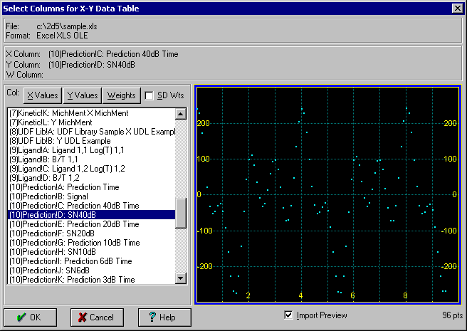
Note that the first two selections are automatically placed in the X and Y positions. You may double click on the column for the Y variable in order to immediately proceed with the read operation. You can also revise the initial X,Y selections as well as to specify a column to be used for the weights. The weights can be optionally imported as standard deviations.

Press OK to accept these choices. Press OK once again within the titles dialog to confirm the imported titles.

This data set consists of the sum of three different sinusoids and 1% Gaussian noise.

Parametric Fitting

Select the Curve Fit Poly/Ratl option in the Process menu or toolbar.

When the fit is concluded, enter the Review by clicking the Graph Start button.

As an alternative, you may press OK and select the Graph Start item in the Review menu. If you do not respond to the conclusion of the fit in 10 seconds, the Review is automatically started.

Using the List menu of the Curve-Fit graph, or the Sort menu of the Equation List, select the Sort by r² item.

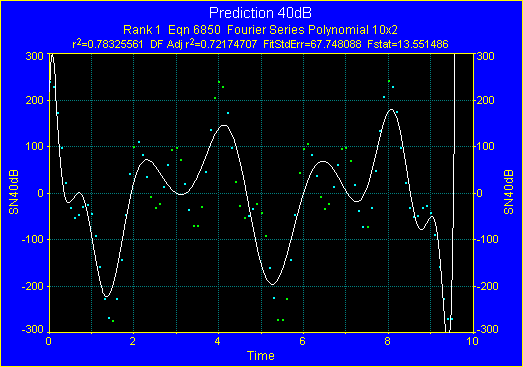
The highest ranked equation, a 21 parameter Fourier series polynomial is unable to map the local minima and maxima in this data set. This is one case where a non-parametric procedure is particularly valuable.

Click OK to close the Review.

Spline Estimation

Select the Spline Estimation option from the Process toolbar or Estimate menu. Select the Cubic algorithm.

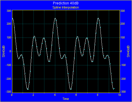
The basic cubic spline does an excellent job interpolating the data.

TableCurve Studio offers a broad selection of spline algorithms. The most common types of splines are cubic splines. These produce smooth first derivatives and continuous (but not smooth) second derivatives.

• • The Cubic option fits a cubic spline interpolant where the breakpoints or knots of the spline are the X values of the data. As such, the knots and order are fixed. The spline passes exactly through each data point.
• • The Cubic constrnd option is similar, except that it minimizes the 'wiggles' common to cubic splines. The wild swings observed when noisy data are fit to cubic splines do not occur with this algorithm. Again, the spline passes exactly through each data point.
• • The Cubic smooth option fits a smooth cubic spline to the data using a automatic smoothing procedure known as cross-validation. Since the interpolant will not pass exactly through the data, TableCurve Studio reports a standard error (SE) and r² for this type of spline.

There are four B-Spline procedures, three of which offer overdetermined least-squares fits.

• • The B-Spline option fits the B-spline of a specified order using a knot sequence based upon the X-values of the data. The knots are thus fixed. Orders range from 2 through order 8. The B-spline passes exactly through each data point. The B-Spline of order 3 is identical to the cubic spline.
• • The LS B-Spline fix option offers a B-spline where the knots are not located at the X-values, but fixed in position, and lower in count than the number of data points. For this option, you must set both the order and the number of knots desired. The smaller the number of knots, the greater will be the smoothing of noisy data. TableCurve Studio reports a standard error (SE) and r² for this type of spline.
• • The LS B-Spline opt option is identical to the previous spline, except that the knots are now variable, and are shifted to further minimize the overall least squares fit. Due to its iterative nature, this algorithm is appreciably slower than all of the other spline options.
• • The LS B-Spline usr option offers a B-spline where the knots are located at user-specified X-values. For this option to be available, a knot sequence must first be imported. You must also specify the spline order.

There is also a NURBS algorithm.

• • The NURBS option fits a non-uniform rational B-spline to the data. The knots are fixed at the X values of the data points. The order can vary from 2 to 8. Unlike the wild oscillations sometimes observed with the higher order B-splines, NURBS become smoother with increasing order. A NURBS by its nature is a smoothing spline, and does not pass exactly through the data points. A standard error (SE) and r² is thus reported.

Although these algorithms suffice for most estimations, TableCurve offers four other estimation procedures. In most cases, you will use one of these other procedures only because the smoothing offered by the above algorithms is inadequate:

• • The best smoothing splines are the least-squares B-splines, but fixed knots do not usually work well, the non-linear optimization that seeks to find the optimum knot sequence may fail, and it can be a tedious process to manually specify a knot sequence.
• • The cross-validation smoothing spline is not useful for derivatives beyond first order.
• • The smoothing offered by NURBS is generally of limited value.

The Smoothed Data Spline Estimation procedure combines TableCurve Studio's automated smoothing with B-spline estimation. The data are pre-smoothed and then fitted to the B-spline. Frequency and eigen domain methods are often superior for removing noise without distorting the underlying deterministic trend.

The Local Regression Spline Estimation option offers a much greater control of the Loess smoothing algorithm. Loess is often very effective when the noise is abysmally high and a data trend is not visually perceptible.

The Savitzky-Golay Spline Estimation option offers a much greater control of the Savitzky-Golay smoothing algorithm and offers interpolation using the constrained cubic spline. This procedure is recommended for estimating derivatives.

The Fourier Estimation option offers Fourier domain filtering with interpolation and smoothed estimations based upon the evaluation of the individual Fourier components.

For more information on the smoothing estimation procedures, please explore the Noise Reduction tutorial.

Since we are not interested in updating the data table, click on Cancel to exit the spline estimation procedure.

Select the Fourier Estimation option in the Estimate menu or Process toolbar.

Unless some form of filtering takes place, all settings will exactly reproduce the input data. The quality of the interpolation, however, will vary.

Be sure Remove Trend is unchecked, set the Window to None, be sure Output Data is set to Function, and change n to 1024.

In the lower graph, use the mouse to zoom-in the region of data between x=8.5 and x=9.5.

Click on the Modify Point Format button in the lower graph's toolbar. Select the Y2 Axis and set the size to 4. Click OK to close the dialog.

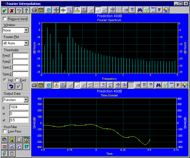
Note the oscillations between the last few data values.

Check the Remove trend box and set the Window to cs3 BHarris 3.

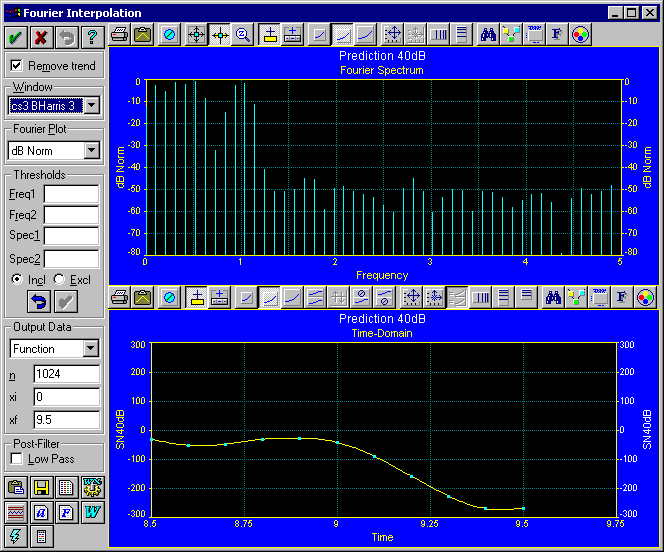
Even though both Fourier decompositions exactly reproduce the input data, they are very different and also produce very different interpolations. The oscillations between the final points are no longer present.

When there is a good indication of a signal-noise threshold, as in this case, it is a simple matter to remove the noise.

Enter -40 for Spec1 and check Excl.

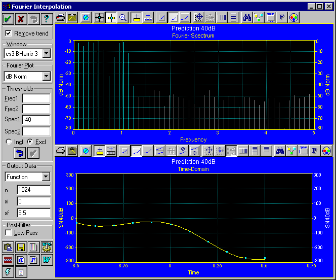
While this removal of the noise may have improved the estimates, note that interpolation is no longer occurring. The Fourier model no longer passes exactly through each data point.

Since we are not interested in updating the data table, click on Cancel to exit the Fourier estimation procedure.

Exit the program by closing the main window or by the Exit item in the File menu.