Eigendecomposition Filtering

This tutorial covers the signal filtering capabilities of TableCurve Studio using Eigendecomposition and reconstruction techniques.

Generating Test Data

Select the Generate Data option in the Edit menu or Main toolbar.

For the Eigendecomposition in this tutorial, we will create a data stream consisting of a sine function, an exponential decay, and white (Gaussian) noise.

Click Read and select the file tutor1.sig from the Data subdirectory.

The following signal expression is imported:

F1=100*EXP(-X/1)

F2=10*SIN(2*PI*X*10)

Y=F1+F2

The X (time) values vary from 0 to 1.0 with a 0.002 sample increment. Gaussian noise is added at a 50% level. The aim is to explore the isolation and recovery of both the sinusoid and the exponential decay.

Click OK to process the current signal.

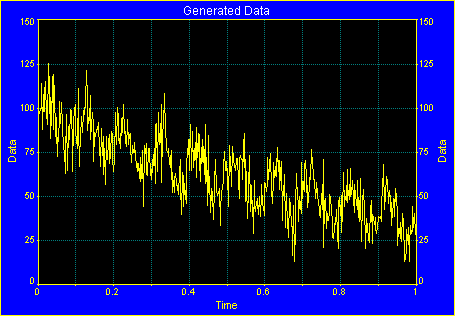
A TableCurve Studio Graph is presented containing the 501 point generated data.

Click OK to accept the generated data. Click Yes when asked to update the main data table with the revised data.

Eigendecomposition Filtration

Unlike Fourier filtering, which isolates components by frequency, Eigendecomposition isolates data components by signal strength. In order for this test case to work, we had to be certain the first order decay had a greater power at all X-values than the sinusoid.

Select the Eigendecomposition Filtering option in the Filter menu or main toolbar. Be sure the CovM FB algorithm is selected, set the matrix order to 60. Also be sure that the Eigenvalues Normalize % box is checked and that Data is checked for the lower graph. Using the left mouse button, box only the first eigenmode in the upper graph.

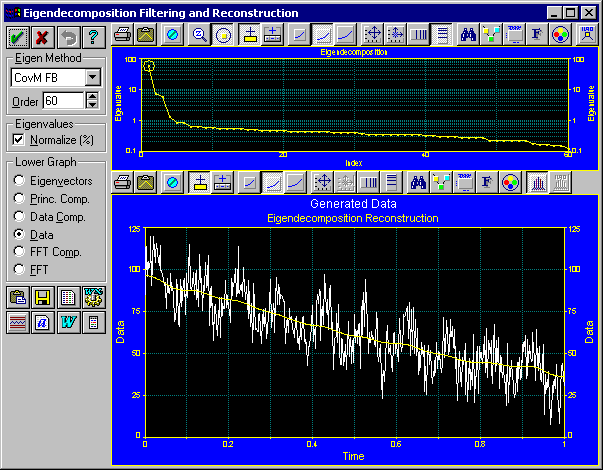
In an eigendecomposition, a continuously increasing or continuously decreasing data component is captured by a single eigenmode. Note that the first order exponential decay is recovered with virtually no trace of the sinusoid.

Click on OK to close the Eigenfiltering procedure and answer Yes to update the data table with this first isolated component.

Select the Curve-Fit Simple Equations option in the Process menu or toolbar. When the fit is concluded, enter the Review by clicking the Graph Start button.

Click on Search for Specific Equation and enter 8157 and click OK.

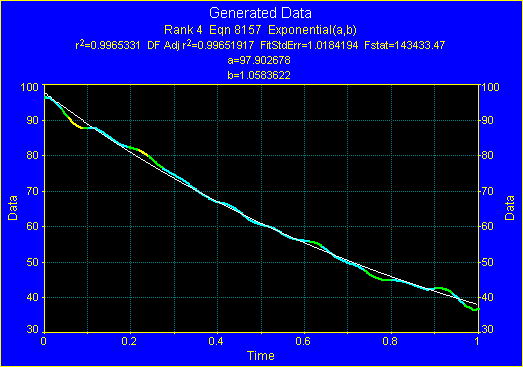
As you will recall, we defined the damped exponential with F1=100*EXP(-X/1). We would thus like to see parameters of (100,1) for the exponential. We are close with (97.9,1.058).

Click OK to close the Review.

Click Reset XY Data to restore the original data.

Again select the Eigendecomposition Filtering option in the Filter menu or main toolbar. Using the left mouse button, box the second and third eigenmodes in the upper graph.

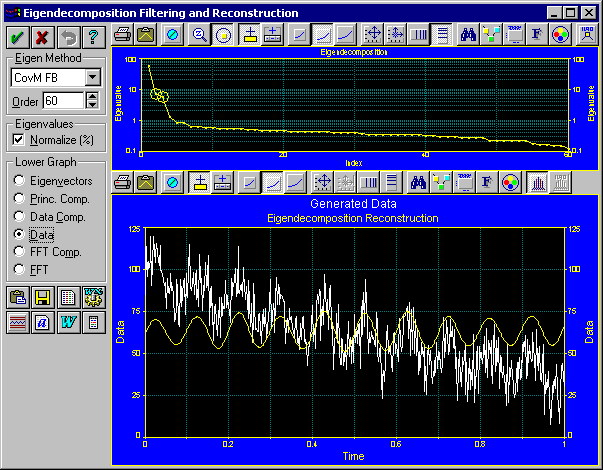
Oscillatory components appear as pairs in an eigendecomposition. Note that the sinusoid is recovered with no presence of the exponential decay.

Check the FFT box and zoom in the spectral peak in the lower graph.

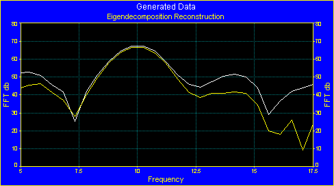
The FFT uses an automatic exact-n FFT procedure with a variable Kaiser-Bessel data taper. Note that the spectral peak's central frequency is at 10. Recall that the sinusoid was generated with F2=10*SIN(2*PI*X*10). The sinusoidal frequency was very accurately recovered.

Right click in the lower graph to restore standard scaling or click on Reset Default Scaling in the graph's toolbar.

Using the left mouse button, box the first, second and third eigenmodes in the upper graph. Check the Data Comp. box.

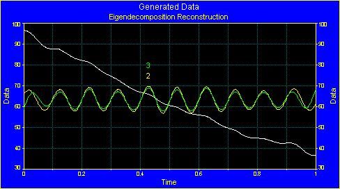
Inspecting the individual components for the first three eigenmodes reveals the completeness of the separation. Bear in mind that a full 50% level of random noise is present in this data set.

Using the right mouse button, again box the first, second and third eigenmodes in the upper graph. Check the Data box.

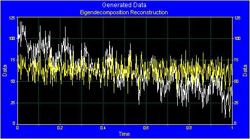
When the right mouse button is used to box the eigenmodes, the enclosed eigenmodes are excluded from the reconstruction. Note that this high level of noise is contained almost entirely in these upper 57 eigenmodes.

Using the left mouse button, again box the second and third eigenmodes in the upper graph. Check the Data Comp. box.

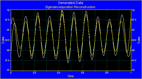
These two components sum to produce the reconstructed sinusoid.

Click on OK to close the Eigenfiltering procedure and answer Yes to update the data table with this first isolated component.

Select the Curve-Fit Waveform Functions option in the Process menu or toolbar. When the fit is concluded, enter the Review by clicking the Graph Start button.

Select equation 8014, the sine-wave model.

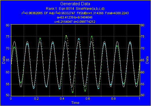
The sinusoid was generated with F2=10*SIN(2*PI*X*10). The sinusoid's amplitude of 10.0 is recovered as 9.55. The phase of 0 (or 2p) is recovered as 1.978p. The frequency of 10 is recovered as 10.02 (1/wavelength). Although the variations in the sinusoidal amplitude suggest a less than ideal isolation, the sinusoid's parameters are recovered quite effectively.

Click OK to close the Review.

Click Reset XY Data to restore the original data.

Parametric Fitting

Select the Process menu’s User Functions item. In the UDF entry screen, enter expsin as the Function Name, 5 as the Adjustable parameter count, Y=A0*EXP(-X/A1)+A2*SIN(2*PI*X*A3+A4) as the UDF expression, and the values 97.9, 1.06, 9.55, 10.02, and 1.978*PI for the five starting estimates.

Click on the Fit UDFs button. When the fit is concluded, enter the Review by clicking the Graph Start button.

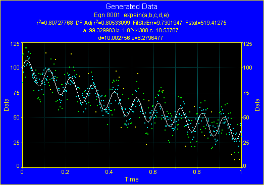
Using the estimates from the two eigenfiltering procedures, the UDF was able to further refine the parameters. Apart from the fact the exponential's amplitude is slightly lower and the sinusoid's amplitude is slightly higher, the generating values are very effectively recovered.

Click OK to close the Review.

Exit the program by closing the main window or by the Exit item in the File menu.