Fourier Filtering
This tutorial covers the Fourier filtering capabilities of TableCurve Studio.
Generating a Test Signal
 Select the Generate Data option in the Edit menu or Main toolbar.
For this tutorial, we will create a data set that contains one reference sinusoid and two low power sinusoids, one with a higher and the other with a lower frequency. The low power components will be -40dB and -60dB below the reference sinusoid. White noise will then be added so that a noise floor exists at approximately -75dB. The object of this test is the accurate frequency and power estimation of these two low power components. A secondary focus will be the recovery of phase information for these components.
Click Read and select the file tutor2.sig from the Data subdirectory.
The following signal expression is imported:
F1=SIN(2*PI*X*1005+PI/4)
F2=0.01*SIN(2*PI*X*505+PI/2)
F3=0.001*SIN(2*PI*X*1505+PI)
Y=F1+F2+F3
The X (time) values vary from 0 to 0.1 with a 0.0001 sample increment. The Nyquist frequency is thus 5000 (half the 10000 sampling frequency). The first low power sinusoid (-40dB) has 1% of the amplitude and 0.01% of the power of one of the reference sinusoid. The other low power test sinusoid (-60dB) has only 0.1% of the amplitude and 0.0001% of the power of the reference sinusoid. The 0.15 Gaussian Noise% creates a white noise floor at about -75dB. It should thus be possible to isolate even the -60dB component given a well designed Fourier filtration.
Click OK to process the current signal.
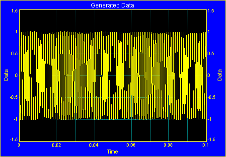
 Click OK to accept the generated data. Click Yes when asked to update the main data table with the revised data. Click OK to accept the default titles.
The 1001 point generated data set is now displayed in the main status window. In TableCurve Studio, the main window is informational only. The various analyses and processing take place in separate procedures that are tailored to each specific option.
Viewing the Data
 Select the View Data option in the Data menu or main toolbar. Zoom in on a region of the data.
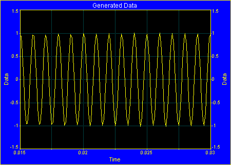
Inspecting the data visually, only the reference sinusoid is apparent. The two low power sinusoids are imperceptible.
Click OK to exit the view option.
Fourier Filtering
 Select the Fourier Filtering option in the Filter menu or main toolbar. Be sure Remove trend is unchecked, set the Window to Chebyshev, the adj parameter to 103, and the edge% to 1.0. Be sure the default Best Exact N algorithm is selected and Nmin is 1001. Select the dB Norm plot.
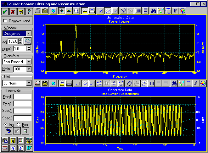
For high dynamic range Fourier spectral analysis, data tapering windows are almost always used. These settings are about optimum for resolving the three components.
 Select zoom-mode and then zoom-in on the three spectral peaks in the upper graph.
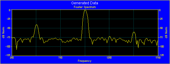
Note that not only are the 505, 1005, and 1505 frequencies accurately resolved, but also the 0dB, -40dB, and -60dB spectral powers.
 Select XY Sectioning mode. Using the left mouse button, box the largest peak down to about -75dB.
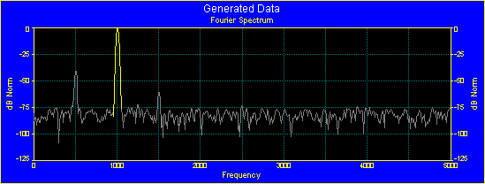
Click on OK to close the Fourier Filtering procedure and answer Yes to update the data table with this first isolated component.
 Select the Curve-Fit Waveform Functions option in the Process menu or toolbar. When the fit is concluded, enter the Review by clicking the Graph Start button.
Select equation 8014, the sine-wave model.
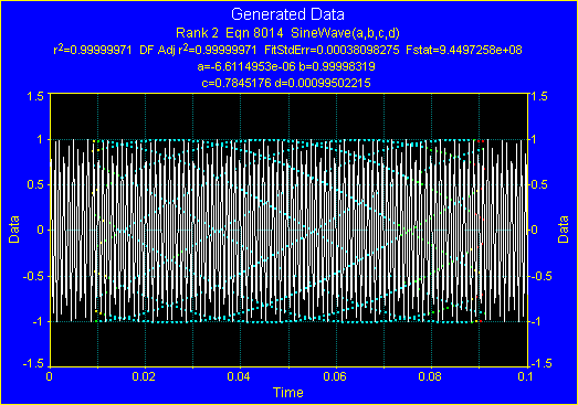
Given this peak's predominance, it is little surprising that the parameters are almost perfectly recovered. The amplitude of 1.0 is recovered as 0.999983, the phase of PI/4 as PI/4.0045, and the frequency of 1005 as 1/0.000995=1005.02. Note that TC2D's built-in sine model computes a wavelength rather than a frequency.
Click OK to exit the Review.
 Click on Reset XY Data to restore the original test data.
Again select the Fourier Filtering option in the Filter menu or main toolbar.
Using the left mouse button, box the lowest frequency peak down to about -75dB. Zoom in on the time domain data in the lower graph.
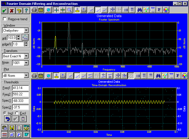
Click on OK to close the Fourier Filtering procedure and answer Yes to update the data table with this first isolated component.
Select the Curve-Fit Waveform Functions option in the Process menu or toolbar. When the fit is concluded, enter the Review by clicking the Graph Start button.
Select equation 8014, the sine-wave model.
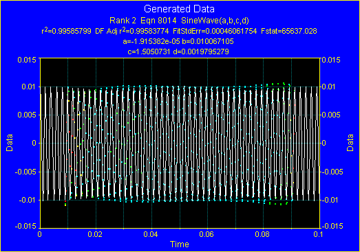
This spectral component has only 1% of the amplitude and 0.01% of the power of the main peak. Still it is recovered with some accuracy. The amplitude of 0.01 is recovered as 0.01001, the phase of PI/2 is recovered as PI/2.087, and the frequency of 505 is recovered as 1/0.001979=505.31.
Click OK to exit the Review.
Click on Reset XY Data to restore the original test data.
Again select the Fourier Filtering option in the Filter menu or main toolbar.
Using the left mouse button, box the lowest power peak down to about -75dB. Zoom in on the time domain data in the lower graph.
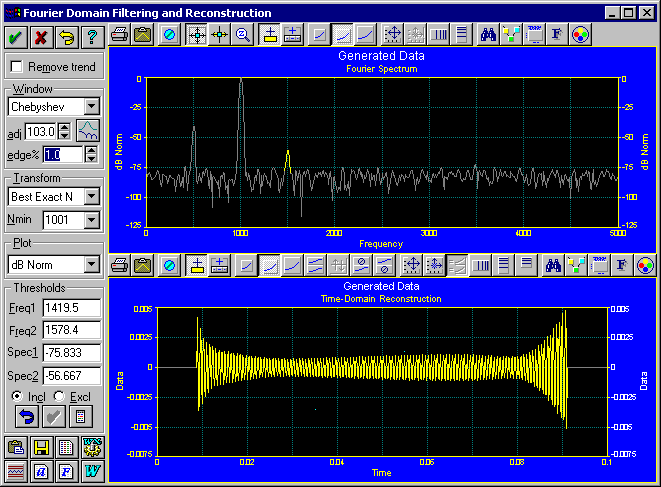
Click on OK to close the Fourier Filtering procedure and answer Yes to update the data table with this first isolated component.
TableCurve Studio currently uses a time domain procedure to scan for estimates of the waveform functions. This procedure works well so long as the number of cycles is not too high. We must thus reduce the number of cycles in the data to be fitted. We must also deal with the anomalies at the edges of the reconstructed data.
 Select the Section Data option in the Data menu or main toolbar.
Enter 0.045 for Xi and 0.5 for Xf. Click on Apply New.
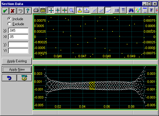
Click on OK to accept the sectioning, answer Yes to deleting the inactive points, and No to saving the old data.
Select the Curve-Fit Waveform Functions option in the Process menu or toolbar. When the fit is concluded, enter the Review by clicking the Graph Start button.
Select equation 8014, the sine-wave model.
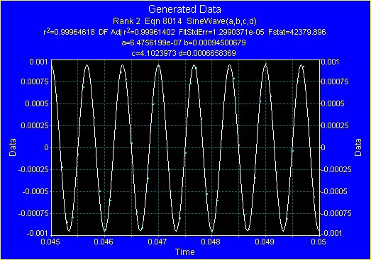
This spectral component has only 0.1% of the amplitude and 0.0001% (1 ppm) of the power of the main peak. Despite this very low presence, the sinusoid is adequately recovered. The amplitude of 0.001 is recovered as 0.00095, the phase of PI is recovered as 1.31*PI, and the frequency of 1505 is recovered as 1/0.000666=1501.5.
Click OK to exit the Review.
Click on Reset XY Data to restore the original test data.
Again select the Fourier Filtering option in the Filter menu or main toolbar.
Linear Sinusoidal Fitting
TableCurve Studio v5 offers linear sinusoidal fitting. The peaks within the frequency spectrum are automatically identified, sorted by power, and up to 25 are automatically fitted to a sum of sinusoids model. In linear sinusoidal fitting, the frequencies are fixed at the values determined in the FFT. For a greater accuracy in these frequencies, a bin interpolation procedure is employed. By fitting a sum of sines and cosines, the phase is also linearized. The linear fitting thus computes the amplitude and phase parameters for the sinusoids at the fixed frequencies found in the FFT.
 Click on the Numeric Summary button.
The frequency analysis is based directly upon the FFT. It finds the three peaks at 505.1005, and 1505 as well as 22 other spectral features within the noise.
Frequency Analysis
Frequency Amplitude Phase Power % Rel %
415.577482 0.00014987 2.41627153 1.1241e-09 4.5002e-06 4.5006e-06
505.098369 0.00712484 1.46921534 2.5407e-06 0.01017120 0.01017225
637.956389 0.00011936 4.09950900 7.1311e-10 2.8548e-06 2.8551e-06
1005.16325 0.70642628 4.77549366 0.02497686 99.9896748 100.000000
1053.48891 0.00015355 3.40435750 1.1801e-09 4.7244e-06 4.7248e-06
1183.81623 0.00011126 3.69921785 6.1951e-10 2.4801e-06 2.4803e-06
1344.91501 0.00012481 3.55058472 7.7969e-10 3.1213e-06 3.1216e-06
1503.78353 0.00066878 3.40847125 2.2385e-08 8.9615e-05 8.9625e-05
1712.07920 0.00010360 3.57119486 5.3715e-10 2.1504e-06 2.1506e-06
2080.27531 0.00013210 2.34054416 8.7343e-10 3.4966e-06 3.497e-06
2179.81897 0.00010370 1.16172654 5.3822e-10 2.1547e-06 2.1549e-06
2256.46209 0.00011913 4.89503962 7.1035e-10 2.8437e-06 2.844e-06
2348.63572 0.00010189 0.51063526 5.1961e-10 2.0801e-06 2.0804e-06
2460.86129 0.00012608 4.46756865 7.9559e-10 3.185e-06 3.1853e-06
2923.33063 0.00010659 3.02230146 5.686e-10 2.2763e-06 2.2765e-06
3124.17822 0.00012836 1.73707390 8.2463e-10 3.3012e-06 3.3016e-06
3303.68903 0.00010463 5.11782383 5.4787e-10 2.1933e-06 2.1935e-06
3484.42147 0.00016586 1.24843320 1.3769e-09 5.5122e-06 5.5127e-06
3696.16562 0.00012169 0.07329151 7.4113e-10 2.967e-06 2.9673e-06
3961.90706 0.00011966 3.45424221 7.1659e-10 2.8687e-06 2.869e-06
4101.96888 0.00012035 3.52112729 7.2495e-10 2.9022e-06 2.9025e-06
4304.92297 0.00010305 1.04096201 5.3145e-10 2.1276e-06 2.1278e-06
4536.10536 0.00010667 0.86048902 5.6951e-10 2.2799e-06 2.2801e-06
4735.07328 0.00010510 1.44313890 5.5287e-10 2.2133e-06 2.2135e-06
4875.93666 0.00010256 1.01889937 5.2645e-10 2.1075e-06 2.1077e-06
0.02497944 100.000000
The linear sinusoidal fit will refine the amplitude and phase parameters for these three components.
Sine Component Fit (Suboptimal)
Frequency Amplitude Phase Power % Rel %
415.577482 0.00042238 4.25431188 8.9305e-09 1.7871e-05 1.7873e-05
505.098369 0.00976607 1.55126979 4.7697e-06 0.00954500 0.00954601
637.956389 0.00026538 3.24608257 3.5253e-09 7.0547e-06 7.0554e-06
1005.16325 0.99965677 0.73405021 0.04996568 99.9893227 100.000000
1053.48891 0.00309756 1.19783156 4.7982e-07 0.00096019 0.00096029
1183.81623 0.00074628 1.14230882 2.7847e-08 5.5727e-05 5.5733e-05
1344.91501 0.00040205 0.65009692 8.0823e-09 1.6174e-05 1.6176e-05
1503.78353 0.00071390 3.22282557 2.5498e-08 5.1026e-05 5.1031e-05
1712.07920 0.00015652 1.89252228 1.2245e-09 2.4505e-06 2.4507e-06
2080.27531 0.00016562 1.41217869 1.3717e-09 2.745e-06 2.7453e-06
2179.81897 0.00012153 0.52004344 7.3849e-10 1.4778e-06 1.478e-06
2256.46209 0.00011887 5.93346461 7.0614e-10 1.4131e-06 1.4133e-06
2348.63572 9.2722e-05 0.34145593 4.3008e-10 8.6066e-07 8.6075e-07
2460.86129 5.5175e-05 2.75591398 1.5216e-10 3.0451e-07 3.0454e-07
2923.33063 7.5954e-05 1.60422938 2.8838e-10 5.7709e-07 5.7715e-07
3124.17822 6.119e-05 3.70163512 1.8725e-10 3.7471e-07 3.7475e-07
3303.68903 0.00015359 0.86178838 1.1798e-09 2.361e-06 2.3613e-06
3484.42147 0.00012083 1.40643256 7.2996e-10 1.4608e-06 1.4609e-06
3696.16562 0.00010446 5.93396454 5.454e-10 1.0914e-06 1.0915e-06
3961.90706 7.933e-05 3.17425105 3.1463e-10 6.2963e-07 6.2969e-07
4101.96888 8.9498e-05 3.78904193 4.0061e-10 8.0169e-07 8.0178e-07
4304.92297 0.00011298 0.91802213 6.3819e-10 1.2771e-06 1.2773e-06
4536.10536 8.8996e-05 1.12938285 3.961e-10 7.9267e-07 7.9275e-07
4735.07328 0.00021892 1.50943628 2.3963e-09 4.7953e-06 4.7958e-06
4875.93666 9.4486e-05 0.33286241 4.4636e-10 8.9323e-07 8.9333e-07
0.04997102 100.000000
r² DOF r² Std Err F-stat
0.9991292255 0.9990586221 0.0216956823 14358.041721
Data Power Model Power Error Power Ratio
0.0500555104 0.0500123879 4.358706e-05 1147.4135605
We will extract these three components for starting estimates in a non-linear 3-sine UDF that we will now fit.
Frequency Amplitude Phase
505.098369 0.00976607 1.55126979
1005.16325 0.99965677 0.73405021
1503.78353 0.00071390 3.22282557
Close the Numeric Summary and then Click on OK to close the Fourier Filtering procedure.
Parametric Fitting
 Select the Process menu’s User Functions item. In the UDF entry screen, enter 3sin as the Function Name, 9 as the Adjustable parameter count, Y=A0*SIN(2*PI*X*A1+A2)+A3*SIN(2*PI*X*A4+A5)+A6*SIN(2*PI*X*A7+A8) as the UDF expression, and the values 0.0098, 505.1, 1.55, 1.0, 1005.2, 0.73, .00072, 1503.8, and 3.22 for the nine starting estimates.
 Click on the Fit UDFs button. When the fit is concluded, enter the Review by clicking the Graph Start button.
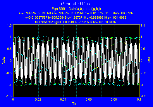
Using the estimates from the linear sinusoidal fitting, the UDF was able to refine the parameters of the sinusoids:
-
- All parameters in the high power component (1,1005,0.7864) are recovered to 5-6 decimal places.
-
- The first low power spectral component (.01,505,1.5707) is recovered as (.01001,505.03, 1.5572).
-
- The lowest power spectral component (.001,1505,3.1416) is recovered as (.00096,1504.66,3.2094)
Click OK to close the Review.
Exit the program by closing the main window or by the Exit item in the File menu.
The Fourier filtering capabilities in TableCurve Studio are drawn from the signal analysis software product, AutoSignal. AutoSignal offers automated harmonic analysis and non-linear optimization with no practical limit on the number of spectral components.