Noise Reduction
This tutorial covers the denoising and smoothing capabilities of TableCurve Studio.
Denoising/Smoothing vs. Curve-Fitting
When fitting a theoretically appropriate parametric model to the trend within a data set, it is not usually desirable to smooth or remove noise prior to fitting. In this particular instance, curve-fitting represents the very finest form of smoothing. As long as the residuals are normally distributed (follow a Gaussian distribution) and lack a systematic trend, the parametric model is a perfectly acceptable way to factor out the noise within a data set. Since a parametric model is also a continuous function, smooth data can be reconstructed at exactly the x values and density desired.
There are instances, however, where the data trend cannot be accurately accounted by a parametric model with a modest number of parameters. Instead, it may be necessary to fit a higher order polynomial or rational function to approximate a complex trend. Here, there are a number of advantages in removing noise prior to fitting. In general, higher order polynomials and rationals tend to fit local trends within the noise. Further, significant noise often results in rational fits with poles (undefined regions) in the x-range of the data. By removing this noise prior to fitting, higher order polynomial and rational fits can be markedly improved.
When there are systematic trends within the residuals of even the best parametric models, the model is insufficient to map the underlying data trend. In this case, one or more of TableCurve Studio's smoothing methods may be more effective in filtering out the noise while minimally impacting the deterministic part of the signal. The Fourier and Eigen domain denoising procedures are often very effective, and unlike parametric fitting, the expertise needed to use these procedures optimally is quite easy to gain.
Smoothing/Denoising, Estimation, and Prediction
In TableCurve Studio, a smoothing or denoising procedure is one where the algorithm always returns smoothed data at the original set of x values. No interpolation or extrapolation is available, and there is no continuous estimation function.
A prediction procedure applies to data with equally spaced x-values and generates estimates at additional discrete x values, at one or both ends of a data stream, as in time-series forecasting. No interpolation occurs and there is no continuous function, although it is possible to estimate or predict an arbitrary number of additional data values with this same x-spacing.
An estimation procedure, on the other hand, is one where the set of x values used for the computation of y values is arbitrary and user-defined. Interpolation is always possible, and as with curve-fit equations, extrapolation or prediction is available, though not always wise. A continuous function, or the means to simulate such, is the central feature of the procedure.
Parametric and Non-Parametric Procedures
In TableCurve Studio, a parametric procedure is one where a set of numeric parameters having intrinsic significance is returned to the user. A non-parametric procedure in TableCurve Studio is one where underlying parameters, if present, are typically intermediates and not generally returned to the user.
Strictly speaking, all procedures are parametric in that some parameter set is is always computed. Instead of equation coefficients, they may be Fourier coefficients, Savitzky-Golay or Kaiser Bessel filter coefficients, eigenvectors and eigenvalues, local regression coefficients, spline coefficients, and so forth.
Smoothing/Denoising and Estimation Analogs
The Filter menu offers procedures that modify the data table by smoothing, removing noise, and isolating components. All of these options return processed data having the original set of x values.
The Estimate menu contains all of TableCurve Studio's non-parametric estimation procedures and also its procedure for AR (autoregressive) prediction. Here the original x values are typically modified, extended in the case of AR prediction and set to interpolation bounds and density for the estimation routines.
Automated Procedures
 The Automated Smoothing option in the Filter menu simplifies the use of six different procedures for smoothing the data table. There include Fourier filtering, Loess, Gaussian convolution, Savitzky-Golay, Eigen filtering, and Kaiser-Bessel filtering. No knowledge of the algorithms is needed and uniform x data are automatically generated when required by an algorithm.
 The Smoothed Data Spline Estimation procedure in the Estimate menu combines automated smoothing and B-spline estimation. These are not smoothing splines, but rather the fitting of an interpolating B-spline to data that have been pre-smoothed.
With only a single smoothing level adjustment, these automated procedures will usually offer a close to optimum level of noise removal for each of the algorithms. In general, distortion of the underlying data trends does not occur until high smoothing levels are specified. In this tutorial, we will begin with the automated procedure. In many instances, its performance will be completely satisfactory.
Specialized Filtering and Estimation Procedures
The more specialized procedures are as follows:
 The separate Savitzky-Golay Smoothing procedure offers much greater control of the Savitzky-Golay algorithm and smooth derivatives through order eight based directly on the smoothing filter.
 The Savitzky-Golay Spline Estimation option additionally adds interpolation with a constrained cubic spline interpolant. This procedure has been especially tailored for estimating derivatives.
 The Local Regression Spline Estimation option offers a much greater control of the Loess algorithm, including higher orders, and also adds interpolation.
 The Fourier Denoising option offers both frequency and signal thresholding for low pass frequency-domain filtration as well as raised data tapers to reduce spectral leakage.
 The Fourier Filtering option additionally offers channel by channel control of the Fourier domain filtering. This routine is generally used for component isolation, although it can be used for lowpass denoising.
 The Fourier Estimation option is a Fourier filtering procedure with interpolation and smoothed estimations based upon the evaluation of the individual Fourier components.
 The Eigendecomposition Denoising option offers a greater control of the algorithm and the means to visually separate the signal and noise eigenmodes via singular value magnitudes.
 The Eigendecomposition Filtering option additionally offers the means to visualize individual or pairs of eigenmodes both in the time and frequency domains. This routine is also typically used for component isolation, although it can also perform signal-noise thresholding.
 The Spline Estimationoption offers eight important spline estimation procedures. Five of these are smoothing splines, a cross-validation cubic, NURBS, and least-squares B-splines.
Prediction
TableCurve Studio offers a single prediction procedure:
 The AR Modeling and Prediction procedure offers effective autoregressive forecasting and extrapolation. The AR algorithms include SVD (singular value decomposition) procedures for in-place noise removal. Multiple orders can be simultaneously plotted and stabilizations are available for roots that lie outside the unit circle. The points that are to be processed can be specified, allowing predictions based on a data segment to be compared with subsequent data. The extent of the prediction is variable and white noise can be added to test the robustness of an algorithm's prediction.
Noise Removal
This tutorial covers the filtering of noise from a data set.
Start TableCurve Studio. Select Start/Programs/TableCurve Studio v5.
 Select the File menu’s Import option (or use the Import button in the main toolbar). If Excel [xls] files are not shown, click on the Files of Type drop-down button and select Excel [xls] files. Select and open the file SAMPLE.XLS.
Select the column with the label (12)Denoising!K: Noise 50% Time to be used as the X-variable in the data table. Select the next column identified in the selection list as (12)Denoising!L: Data for the Y-variable. Check Import Preview to see a graph of the data that will be imported.
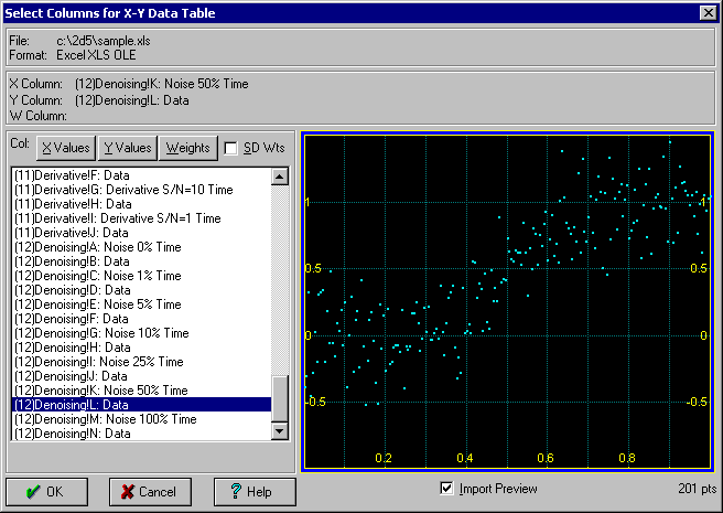
Note that the first two selections are automatically placed in the X and Y positions. You may double click on the column for the Y variable in order to immediately proceed with the read operation. You can also revise the initial X,Y selections as well as to specify a column to be used for the weights. The weights can be optionally imported as standard deviations.
Press OK to accept these choices. Press OK once again within the titles dialog to confirm the imported titles.
This data was generated from a sigmoid model with (1,0.5,0.075) parameters. 50% Gaussian (white) noise was added. This means that the SD of the noise is half the SD of the clean signal.
Parametric Fitting
 Select the Process menu's Curve Fit Transition Functions. Click on Clear. Select Sigmoid. Select the Only Zero Intercept Versions (no constant) control.
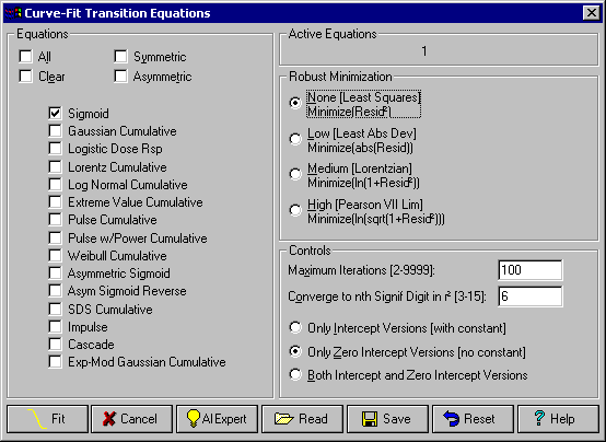
 Click the Fit button.
When the fit is concluded, enter the Review by clicking the Graph Start button.
 As an alternative, you may press OK and select the Graph Start item in the Review menu. If you do not respond to the conclusion of the fit in 10 seconds, the Review is automatically started.
Parametric Smoothing
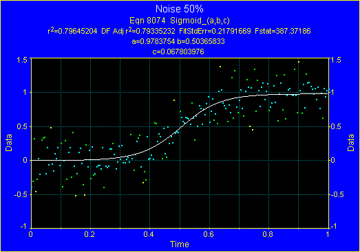
The Curve-Fit graph reveals a very good recovery of the coefficients. The amplitude of 0.978 compares favorably to the 1.0 in the noise-free data. The transition center of 0.504 is very close to 0.5, and the transition width of 0.068 is somewhat sharper than the 0.075 used to generate the data. The errors are 2.2%, 0.72%, and 9.6%.
Marking Outliers and Refitting
 Click on the Mark Excluded Points for Refit option. Select All Points Outside 2 Standard Errors and click OK. Acknowledge that 10 points will be excluded.
The marked points will be toggled in state (in this case disabled or turned off) when a refit is made.
Click on the Refit Transition Equations and UDFs button just to the left.
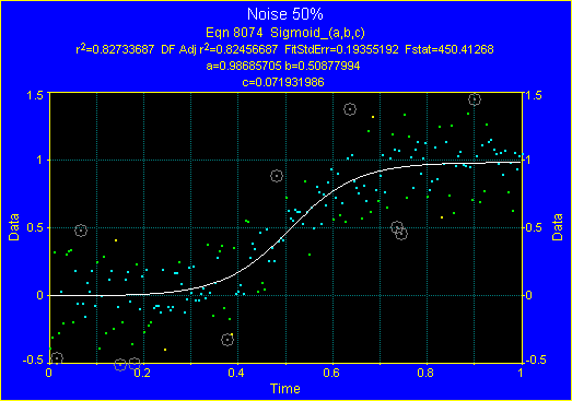
By removing the largest outliers from the fit, the coefficient recovery is improved. The coefficients of 0.987, 0.509, and 0.072 represent errors of 1.3, 1.7, and 4.1% from the noise-free values.
To reactivate all points, once again click on the Refit Transition Equations and UDFs button.
 Click OK to close the Review.
Automated Smoothing
Select the Automated Smoothing option from the toolbar or Filter menu.
With the exception of the Loess procedure, all of the algorithms in the Automated Smoothing option require uniformly spaced data. If a constant x spacing is not present, this procedure automatically generates uniform data for all of the algorithms except Loess. A constrained cubic spline interpolant is used. This is not a factor for this data set since uniform x spacing is present.
Select the FFT Filtering algorithm and click on the AI Expert button.
Select the Loess algorithm and click on the AI Expert button.
Select the Savitzky-Golay algorithm and click on the AI Expert button.
Select the Gauss Convol. algorithm and click on the AI Expert button.
Select the Eigendecomp. algorithm and click on the AI Expert button.
Select the Kaiser-Bessel algorithm and click on the AI Expert button.
This is a very difficult data set to smooth because of the high noise level and a transition function's unique mix of straight line and curved regions. We will list the results for all six, although for this tutorial we will proceed with the one algorithm that best preserves the transition shape visually.
Select the Eigendecomp. algorithm. Click the OK button. Answer Yes to update the data table.
Select the Process menu's Curve Fit Transition Functions and click the Fit button. When the fit is concluded, enter the Review by clicking the Graph Start button.
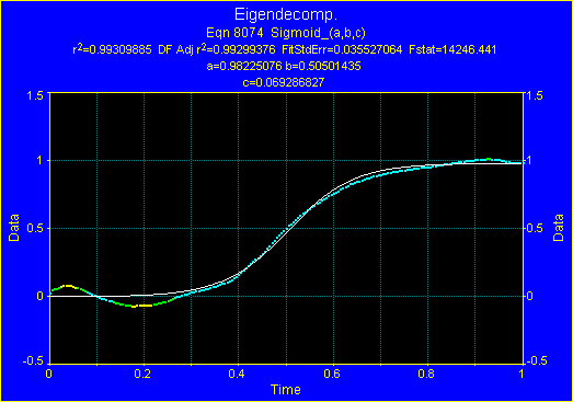
The coefficients of 0.982, 0.505, and 0.069 represent errors of 1.8, 1.0, and 7.6% from the noise-free values.
Comparing the Algorithms
To create a simple appraisal, we will average together the errors for the three coefficients.
Parametric, all points (0.9783, 0.5037, 0.0678) ParmErr=4.17% r²=0.7965 EqNoise=57.8%
Parametric, excl 2SD+ (0.9869, 0.5088, 0.0719) ParmErr=2.40% r²=0.8273
FFT Filtering (0.9796,0.5039,0.0680) ParmErr=4.05% r²=0.9776 EqNoise=0.182%
Loess (0.9782,0.5045,0.0709) ParmErr=2.85% r²=0.9946 EqNoise=0.195%
Savitzky-Golay (0.9817,0.5044,0.0683) ParmErr=3.88% r²=0.9871 EqNoise=0.181%
Gaussian Deconv. (0.9546,0.4950,0.0635) ParmErr=6.96% r²=0.9759 EqNoise=0.179%
Eigendecomp. (0.9822, 0.5050, 0.0693) ParmErr=3.46% r²=0.9931 EqNoise=0.294%
Kaiser-Bessel (0.9867, 0.5058, 0.0700) ParmErr=3.05% r²=0.9915 EqNoise=0.179%
Apart from the small attenuation observed with the Gaussian Deconvolution smoothing, the parametric fit of the smoothed data produces parameter values very close to that of the least-squares sigmoidal fit of the unsmoothed data. The high r², particularly with the Loess and Eigendecomposition algorithms, indicates a very high level of smoothing was achieved while minimally impacting the underlying data trend. The smoothing algorithms included within TableCurve Studio have been selected for their robustness and effectiveness. They represent the best in noise removal technology.
The Equivalent Noise % uses a time domain polynomial interpolation procedure for estimating the Gaussian noise in a data set. The 57.8% white noise estimate for the raw data compares favorably with the 50% noise actually added. All of the procedures filtered out at least 99.5% of the noise originally present.
Here are the curve-fits from the other five procedures:
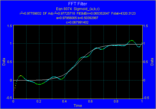
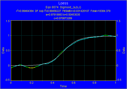
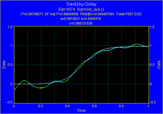
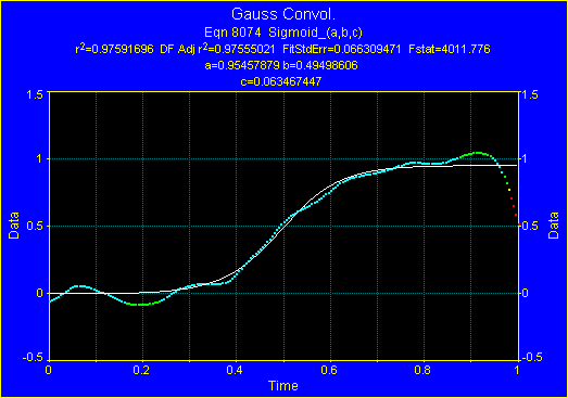
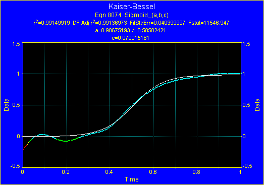
The AI Expert in the Automated Smoothing seeks to select reasonable smoothing levels. It cannot select an optimum. Visually, there is at least a promise that the FFT and Savitzky-Golay procedures could be further optimized.
Click OK to close the Review.
 Click the Reset XY Data to restore the unsmoothed data.
Savitzky-Golay Smoothing
Select the Savitzky-Golay Smoothing procedure from the main toolbar or Filter menu.
Set the one-sided size of the moving window (Win n) to 32. Set the Order to 2 for quadratic fitting and set the sequential pass count (Passes) to 3. Be sure Data is selected.
Note that the quadratic does a better job of managing the straight line portions of the transition.
Click OK to close the procedure. Answer Yes to update the data table.
Again select the Process menu's Curve Fit Transition Functions and click the Fit button. When the fit is concluded, enter the Review by clicking the Graph Start button.
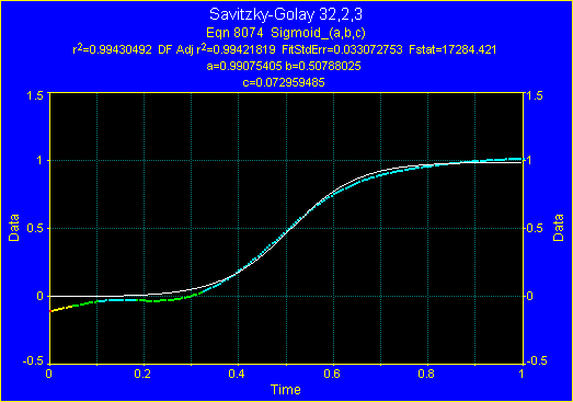
Savitzky-Golay (0.9817,0.5044,0.0683) ParmErr=3.88% r²=0.9871 EqNoise=0.181%
Savitzky-Golay Opt. (0.9907,0.5078,0.0729) ParmErr=1.74% r²=0.9943 EqNoise=0.177%
The optimized algorithm offers a significant improvement in noise reduction and better recovers the underlying parameters.
Click OK to close the Review.
Click the Reset XY Data to restore the unsmoothed data.
Select the Fourier Denoising option in the Filter menu or main toolbar.
Experiment with different windows (data tapers). Explore both Frequency and dB thresholds. Graphically set the thresholds by clicking at the frequency or signal magnitude desired.
Fourier denoising depends on the ability to attribute all spectral information beyond a certain frequency or below a certain spectral threshold to noise. Because of spectral leakage from edge effects and components failing to center within a frequency bin, the signal is not likely to be conveniently confined to certain bins while noise is confined exclusively to the remainder. In practice, the signal/noise separation is incomplete.
Finding a good signal-noise threshold, either in frequency or signal strength, is not easy with this data set. You will probably be disappointed. Sums of sinusoids do not easily map a mix of curves and straight line regions within a data stream.
 Click Cancel to close the procedure.
Eigendecomposition Denoising
An eigendecomposition uses adaptive non-parametric basis functions, partitioning a data stream by signal strength rather than frequency. The highest power components distribute amongst the initial eigenmodes while the noise is found in the subsequent eigenmodes. Denoising using eigendecomposition procedures is often the best way to remove noise from data, provided a high enough matrix decomposition order is possible.
A single eigenmode will capture a continuously increasing or continuously decreasing component within a data stream. An exponential decay, for example, is captured by a single eigenmode. Two eigenmodes are needed to capture a transition since the slope is not continuously increasing or decreasing. Two eigenmodes are also needed to capture an oscillation of a given frequency. That oscillation can be a sinusoid, an exponentially damped sinusoid, a sawtooth, a square wave, or any other shape. If the amplitude of the oscillation varies in accord with a continuous function of time, the two eigenmodes will still map this oscillation. On the other hand, variable frequency oscillations such as chirps may require a large number of eigenmodes to fully map the non-stationary data trend.
Select the Eigendecomposition Denoising option from the Filter menu or main toolbar. Be sure the CovM FB (forward-backward covariance matrix) algorithm is selected and set the Order of the eigendecomposition matrix to 70. To accommodate the single transition, set the Signal Space to 2.
Note that you can set the signal space graphically by selecting the last eigenmode representing signal. Do not include eigenmodes that are part of the long sloping noise floor.
Click OK to close the procedure. Answer Yes to update the data table.
Once again, select the Curve Fit Transition Functions item and click the Fit button. When the fit is concluded, enter the Review by clicking the Graph Start button.
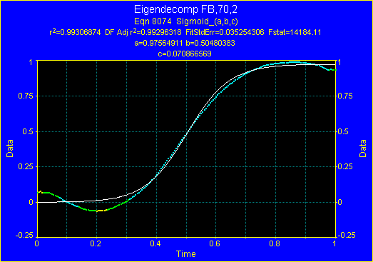
Eigendecomp. (0.9822, 0.5050, 0.0693) ParmErr=3.46% r²=0.9931 EqNoise=0.294%
Eigendecomp. Opt (0.9756, 0.5048, 0.0709) ParmErr=2.96% r²=0.9931 EqNoise=0.236%
The higher order eigendecomposition allowed for more of the noise to be captured and discarded. In the automated smoothing, the eigendecomposition's order is never greater than 40. In this instance, a model order of 70 means that 68 eigenmodes are available to capture and discard noise, rather than 38. This higher level of denoising resulted in a better recovery of the underlying parameters, although the goodness of fit was not improved because of the larger oscillation on the lower plateau of the transition.
Click on OK to exit the Review. Exit the program by closing the main window or by the Exit item in the File menu.