Fitting Parametric Functions

This tutorial focuses upon the task of finding a parametric model for a data set. In a parametric model, the main emphasis is upon solving for the parameters that are intimately associated with features within the data. Unlike approximating functions intended only for interpolations and extrapolations, a parametric model is very sensitive to parameter count and to interactions between the parameters.

Parametric Functions

A parametric model need not have an underlying theoretical foundation, although such is frequently the case. When there is a theoretical underlying model, each of the parameters represents a physically or theoretically real quantity such as energy, concentration, time, temperature, and so forth.

A parametric model with an underlying theoretical foundation relates the dependent variable Y to the independent variable X via a postulated physical relationship between them.

Often a parametric model is used not for describing an underlying theoretical model but rather for characterizing the unique features within a data set. The data set used in this second tour is of this type. Here features of the data are known to have a direct relationship with the underlying physics, chemistry, biochemistry, physiology, or human factors, but there is no quantitative underlying theoretical model.

This type of analysis, which treats the system producing the data as a "black box", results in parameters that can be used to infer trends or characteristics. No better example exists than human biochemistry whose complexity often precludes the availability of a theoretical model. The example that follows should clearly demonstrate the nature of this type of parametric curve-fitting.

Importing A Pharmacological Data Set

Start TableCurve Studio. Select Start/Programs/TableCurve Studio v5.

Select the File menu’s Import option (or use the Import button in the main toolbar). If Excel [xls] files are not shown, click on the Files of Type drop-down button and select Excel [xls] files. Select and open the file SAMPLE.XLS.

To aid in the identification of the columns, TableCurve Studio lists the string data existing in the first 100 rows of the individual sheets or pages in the worksheet file. You must have at least one entry within the first 100 rows of a column in order for that column to be available for selection.

Select the third column with the label (2)Sample2!A: Tour 2: Parametric Functions to be used as the X-variable in the data table. Select the fourth column identified in the selection list as (2)Sample2!B: Concentration for the Y-variable. Check Import Preview to see a graph of the data that will be imported.

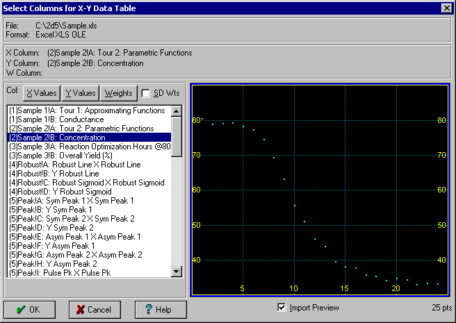
Note that the first two selections are automatically placed in the X and Y positions. You may double click on the column for the Y variable in order to immediately proceed with the read operation. You can also revise the initial X,Y selections as well as to specify a column to be used for the weights. The weights can be optionally imported as standard deviations.

Press OK to accept these choices. Press OK once again within the titles dialog to confirm the imported titles.

The selected columns of data are read and a summary is given for the read operation. 25 data points are read.

Note that a background thread fitting may automatically occur as soon as the data is imported, depending on the Background Thread Processing option currently selected. For the purpose of this tutorial, we will ignore any background thread fitting that takes place.

X=0,Y=0 Data

The first data pair, which has an x value of 0.0, is included in the data set. Although TableCurve Studio substitutes 1E-25 for 0.0 in an effort to keep all logarithmic and inverse equations available, it is usually best to exclude all x=0 points (and y=0 as well if fitting lny or 1/y equations) unless the point has real significance. As you will note here by looking at the first few data points, this x=0 measurement is not needed because the upper plateau is represented adequately by the subsequent points. As such, we will first exclude this initial point prior to fitting.

TableCurve Editor

TableCurve Studio offers two numeric editors and also the means to graphically edit data. The TableCurve Editor offers a simple spreadsheet-like form of editing, while the ASCII Editor offers the ability to edit the data table in a Notepad-style of editor.

In the Data menu’s Section Data option, points can be toggled on and off simply by clicking on them. For this tutorial, we will exclude the point in the TableCurve Editor.

Select the Edit menu’s TableCurve Editor option. Check the Ex (Exclude) box for point #1 and press OK. You may answer No to the prompt for saving the revised data.

The TableCurve Studio status window will now show 24 rather than 25 active points and in the graph, the first point will be shown in the inactive color.

At time=0, the species under study had a concentration of about 80 units. This corresponds to the level in the bloodstream after injection. After some hours, the level begins to drop and goes through an S-shaped transition to a final value near 35 units that represents the level of species normally present.

Transition Functions

Such transitions, while frequent in pharmacology, are found in virtually every science. Often they are positive in their slope rather than negative. The equations describing this type of data trend are often referred to as transition, S-shaped, or cumulative functions.

In this example, the models being fitted will not address the underlying biochemistry. What is important is that the models each offer the following parameters:

• • Concentration at the upper or lower plateau
• • Height of the transition in concentration units
• • Time value for the center of the transition
• • A transition width, slope, or steepness factor that characterizes how rapidly the transition occurs
• • If needed, a parameter that characterizes the asymmetry present in the transition

Note that such parametric models offer a meaningful way to map the essential features of the data. The scientist can then use this type of model in repeated experiments to see how various biochemical factors might affect one or more of these fitted parameters.

Fitting The Transition Functions

You can use the Help menu’s List Equations item to display the full equation set. The transition functions are near the bottom of the list within the non-linear equations. Specific mathematical properties of these models are given in the Transition Functions section of the help system and in the NONLINEQ.PDF Adobe Acrobat document included in the product distribution.

TableCurve Studio offers 29 built-in non-linear transition function equations, zero-intercept and intercept forms of 14 different transition models and an impulse model. Of the 15 individual models, 5 produce a symmetric transition and 10 produce an asymmetric one.

For this example, we wish to fit only these non-linear transition functions. Linear models, particularly rational equations, can fit this data very effectively, but they are approximating functions only, and the coefficients will not yield the desired parameters which describe the essential features within the data.

In the intercept form of the transition functions of interest, the a term represents the lower plateau, b the height of the transition, c the center of the transition, and d describes the steepness of the transition.

Customizing TableCurve Studio’s Transition Function Fitting

TableCurve Studio offers separate customizations for fitting its peak, transition, and kinetic functions. Each of these configurations places all pertinent controls and function selection information in a single place. These options also offer an AI Expert option which will scan the profile of the data and suggest recommended equations.

Select the Process menu’s Curve-Fit Transition Functions and then click the AI Expert button.

The AI Expert option suggests that it would be a waste to bother with symmetric transitions, since the data were found to have a clear asymmetric nature. This option also suggests the fitting of only the intercept version of the functions since neither plateau is anywhere near zero.

Non-linear fitting is iterative, and as such, the maximum number of iterations permitted for a non-linear equation, as well as the convergence criteria, are selectable. The default value of 100 should be sufficient for all except complex UDFs with poor starting estimates.

The default convergence precision of 6 means that the r² must be unchanging in the sixth significant figure for 5 consecutive iterations to signal convergence.

Since there are no apparent outliers in this data set, no reason to believe that errors are other than normally distributed, and only a modest Y-range, there is no reason to use a robust minimization.

For the purpose of this tutorial, we will add a symmetric transition function.

Click on the Gaussian Cumulative function.

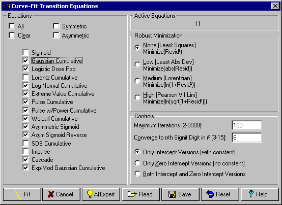
Press Fit to initiate the fitting of these functions.

This should require less than a second on a Pentium machine. Ten equations are successfully fitted.

When the fit is concluded, enter the Review by clicking the Graph Start button.

As an alternative, you may press OK and select the Graph Start item in the Review menu. If you do not respond to the conclusion of the fit in 10 seconds, the Review is automatically started.

Reviewing The Transition Equations

Using the List menu of the Curve-Fit graph, or the Sort menu of the Equation List, select the Sort by F-statistic item.

For parametric functions, you will almost always want to use the F-statistic sort method which orders the equations based upon how accurately a given model can be said to describe the data.

We will first insure that we are using the simpler notational format for non-linear models. Some of the non-linear transition models are rather complex and produce long titles.

Select the Preferences item in the Curve-Fit Graph’s File menu and be sure that the Notational Format for Non-Linear Equations option is checked. Press OK.

To better see the various goodness of fit indices within the ranked ordering, we will display all four criteria within the Equation List.

Using the List menu of the Equation List window or the List menu of the Curve-Fit Graph, select the All Goodness of Fit in List option.

Extreme Value Cumulative

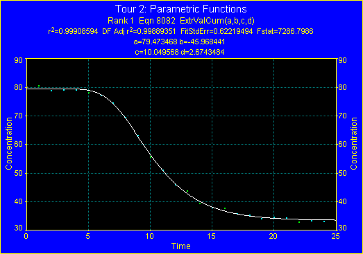
The highest ranked equation by F-statistic is the four-parameter Extreme Value Cumulative equation. This is clearly a model that fares very well in fitting this data. The higher the F-statistic, the more accurately a given model can be said to describe the data. The F-statistic of this equation is 7287, quite good given the noise in the data.

Note that the third-ranked Asymmetric Sigmoid with Reverse Asymmetry, a 5-parameter equation, offers a higher r² and a lower Standard Error.

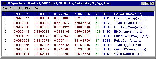
The F-statistic suggests the Extreme Value Cumulative is the superior model since it essentially accomplishes with four parameters what the Asymmetric Sigmoid with Reverse Asymmetry requires five to achieve, although it offers the best least-squares fit in doing so.

Scanning Equations

Use the arrow buttons in the Curve-Fit Graph to inspect the other eight equations in the list.

Scanning can also be done by clicking on the equation desired in the Equation List, by using cursor keys if the Equation List window has the active focus, or by selecting items in the Scan menu of the Curve-Fit Graph. If the Curve-Fit graph window is active and you have a scroll-wheel mouse, you can scroll the equations using the mouse wheel.

The curve-fit graphs for the asymmetric transition models are largely indistinguishable except for the indication of the undefined condition at 0 for the Logistic Dose Response and Log Normal Cumulative and the sharp initiation of the transition for the Pulse Cumulative and Weibull Cumulative. To more readily see the differences we will lock the Extreme Value Cumulative as a reference.

Fit Reference

With the Extreme Value Cumulative selected, click the Add Current Equation as Reference button (or the Add Current Equation as Reference in the Reference menu).

Initially, the reference and current curve will be identical, overlapping one another.

Use the arrow buttons to inspect the other equations against relative to this reference.

The subtle differences should be much more apparent.

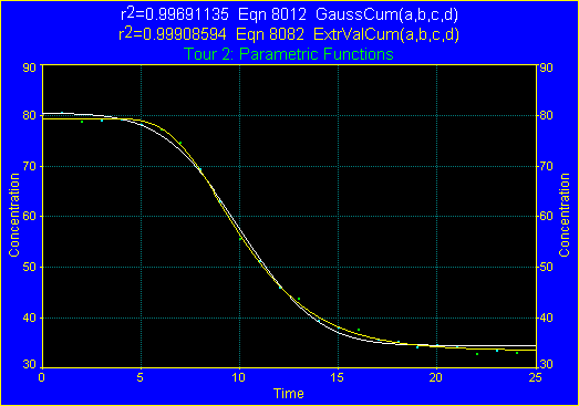
Use the Toggle Display of Equation References button to disable the display of the references.

Use the double up arrow button to return to the Extreme Value Cumulative equation.

Confidence and Prediction Intervals

The confidence intervals are a measure of how accurately the average curve for repeated experiments is determined. The prediction intervals measure how accurately an individual curve is determined relative to the next experiment’s expected values. The prediction bands will always be wider than the confidence bands. We will assume this data represents the average of a considerable number of trials, and as such, we will use only the confidence intervals.

Click on the Set Confidence/Prediction Intervals, %Confidence button in the graph’s toolbar. Be sure the Confidence type of interval is checked, the Prediction type of interval is unchecked, and that the 99% level is checked. Click OK.

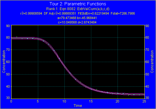
Scan through the equations noting the breadth of the confidence intervals for each equation.

Note the widening of the interval at the sharp initiation of the Weibull transition.

When finished, toggle the intervals off using the Show Confidence/Prediction Intervals button and re-select the Extreme Value Cumulative equation.

Residuals

Click on the Resid button to display the residuals for the Extreme Value Cumulative fit. Scan though the equations noting the degree of randomness of the residuals for each.

The number appended to the Y title is the runs count, the number of times the residuals display a sign change across the X range. You will note that while all of the equations produce little in the way of a systematic trend, the runs count is highest for the Asymmetric Sigmoid with the Reverse Asymmetry, the equation with the smallest fit standard error.

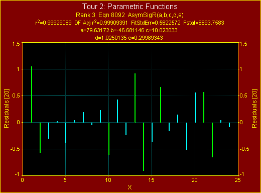
When systematic trends are observed in the residuals, it is usually an indication of an inappropriate or incomplete model. Note the clear systematic trend on the Gaussian cumulative, the symmetric transition model we added to the equation set:

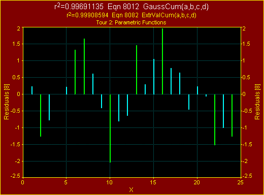
The residuals must be normally distributed in order for the standard errors and confidence statistics to be valid.

Stabilized Normal Probability Residuals Plot

Using the toolbar in the Residuals Graph, click on the Display Residuals in Stabilized Normal Probability Plot button.

Note that the residuals format buttons are also displayed on the left side of the dialog.

On a delta SNP graph, perfectly normal residuals plot as a y=0 line and critical limit lines plot as horizontal lines above and below. TableCurve Studio plots 90%, 95%, 99%, and 99.9% critical limit lines. The 99% critical limit means that in only 1 out of 100 data sets should even a single point appear outside the limit.

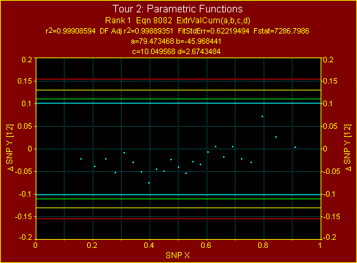
In this case, all points are easily within even the 90% limit for all of the fitted equations, readily confirming this assumption of Gaussian errors.

Click on the Display Basic Residuals button to restore the traditional format.

Close the Residuals window either directly or by again pressing the Resid button in the control panel of the Curve-Fit Graph.

If it is not currently selected, click on the top-ranked Extreme Value Cumulative equation in the Equation List.

Numeric Summary

Click on the Numeric button to open a numeric summary of the Extreme value Cumulative fit. Scroll to the parameter table.

Rank 1 Eqn 8082 ExtrValCum(a,b,c,d)

r² Coef Det DF Adj r² Fit Std Err F-value

0.9990859398 0.9988935060 0.6221949450 7286.7986262

Parm Value Std Error t-value 99% Confidence Limits P>|t|

a 79.47346826 0.281909107 281.9116744 78.67134111 80.27559541 0.00000

b -45.9684411 0.413311267 -111.219908 -47.1444520 -44.7924301 0.00000

c 10.04956768 0.062296479 161.3183907 9.872313038 10.22682232 0.00000

d 2.674348365 0.076175292 35.10781902 2.457603788 2.891092942 0.00000

Area Xmin-Xmax Area Precision

1212.0510118 1.4381e-17

Function min X-Value Function max X-Value

33.677619403 24.000000000 79.473468201 1.0000017963

1st Deriv min X-Value 1st Deriv max X-Value

-6.323351375 9.0693820931 -4.679e-07 1.0000015911

2nd Deriv min X-Value 2nd Deriv max X-Value

-1.986044726 6.4955283716 1.0355597619 11.643241597

Procedure Minimization Iterations

LevMarqdt Least Squares 7

r² Coef Det DF Adj r² Fit Std Err Max Abs Err

0.9990859398 0.9988935060 0.6221949450 1.1885317988

Source Sum of Squares DF Mean Square F Statistic P>F

Regr 8462.7396 3 2820.9132 7286.8 0.00000

Error 7.742531 20 0.38712655

Total 8470.4822 23

Date Time File Source

May 5, 2000 9:31:39 PM c:\2d5\tour2.sav

The t-values are nothing more than the parameter values divided by their standard errors. These t-values can serve as indicators of the degree of certainty with which the parameters are determined. Here the upper plateau of the transition is determined with the greatest certainty. The steepness or width of the transition was determined with the least certainty. The standard errors and confidence limits are still quite good for pharmacological data.

The Options menu offers the means to toggle on and off the different elements of the Numeric Summary.

The Gaussian Quadrature method, with a 1E-8 target precision, is used for the area of the function from Xmin to Xmax. Brent’s method is used for the function and derivative extrema. Note that the X value for the first derivative minimum is the center for the underlying Extreme Value peak. All TableCurve Studio transition functions report a true X50, the X value at 50% of the transition. Only for symmetric transitions will the X50 equal the center of the underlying peak.

Scroll the numeric window so that the parameter table is displayed and then scan down two equations (or directly select the Asymmetric Sigmoid Rev equation).

Rank 3 Eqn 8092 AsymSigR(a,b,c,d,e)

r² Coef Det DF Adj r² Fit Std Err F-value

0.9992908869 0.9990939110 0.5622571952 6693.7582600

Parm Value Std Error t-value 99% Confidence Limits P>|t|

a 79.63171966 0.299006021 266.3214590 78.77628301 80.48715630 0.00000

b -46.6811462 0.415867559 -112.250031 -47.8709161 -45.4913764 0.00000

c 10.02303344 0.057336511 174.8106630 9.858997440 10.18706945 0.00000

d 1.025013498 0.110559341 9.271161411 0.708710462 1.341316534 0.00000

e 0.299893428 0.046812693 6.406241693 0.165965378 0.433821479 0.00000

Note the smaller t-values and the wider confidence limits, and the same trend as to which parameters are most accurately determined. Here, though, there are two width terms and neither is determined with a great deal of certainty. For the F-statistic to increase with an additional parameter, that parameter must make a significant contribution to improving the overall fit. In this example, there is no evidence to support the use of a five parameter model.

Close the Numeric window and select the Extreme Value Cumulative equation.

Data Summary

The Data option displays a point by point data summary with residuals, confidence limits, and prediction limits.

Use the Data button in the Curve-Fit graph control panel to open a Data window. Note the information available and then close the window, either directly or by again using the Data button.

Derivatives and Cumulative Areas

Click the Toggle First Derivative on Y2 Axis in the Curve-Fit Graph’s control panel.

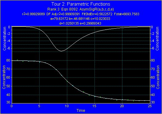
The first derivative curve is an inverted Extreme-Value peak shape since this peak is the derivative of the Extreme-Value Cumulative.

One-to-One Fit and Residuals

To see the Residuals and Fit together, click the Toggle Residuals on Y2 Axis button.

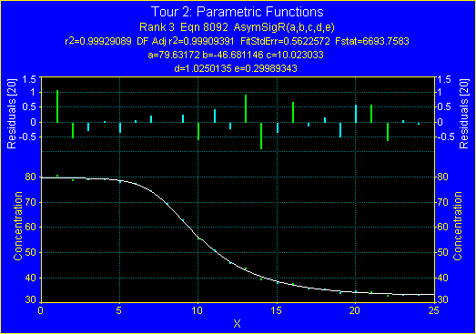
Click the Toggle Residuals on Y2 Axis button to turn off the Y2 residuals and then click.

Click OK to exit the Review.

User-Defined Functions

Let us assume an inventive pharmacologist wanted to see if the models associated with the throughput in a chromatographic column would have any applicability to this biochemical disappearance of this drug in the human bloodstream. Drugs often bind to various molecular sites in ways that could possibly be analogous to the chromatographic mechanisms.

The Exponentially-Modified Gaussian and the Haarhoff-VanderLinde equation are two popular chromatographic peak models. We will use TableCurve Studio’s UDF feature to fit cumulatives of these two models to this pharmacological data. TableCurve Studio can store its UDFs in single files, or multiple files can be saved to UDF libraries. Here we will load a library that contains the Cumulative EMG and Cumulative HVL models.

Although TableCurve includes the Cumulative EMG model in its built-in set, we will also fit this same model using a UDF.

Select the Process menu’s User Functions item. In the UDF entry screen, click on the Read UDF Library item and then select the UDF file SAMPLE01.UDL. Click OK.

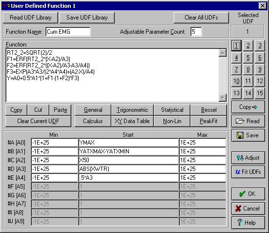
The user functions each use A0, A1, A2, etc. for the adjustable parameters. The Cumulative EMG is a rather complex five-parameter model. In this UDF, parameter formulas are used to make the UDF applicable to any range of X and Y data. TableCurve Studio uses specific rules for constructing UDFs. Many of these exist to assist the UDF compiler in producing equations that run nearly as fast as built-in equations.

UDF Auto Adjust

To insure a successful convergence in the non-linear fit, press the Adjust item. Rather than adjust individual parameters, use the Find & Update item to automatically improve the estimates.

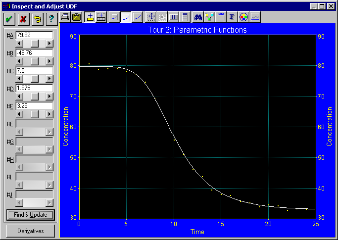
Press OK once the estimates have been refined and answer Yes to replacing the formulas with the revised numeric values.

So long as UDFs will not be saved back to disk, these modifications are one-time only adjustments.

The 1-15 numeric keypad in the dialog is the control center for selecting from among TableCurve Studio’s 15 UDF equations that can be active at any given time. The Cumulative HVL equation was previously saved in position 2 of the UDF library.

Click on the 2 button to change to the second UDF.

There may be a small delay as the first UDF is validated and compiled. Note that the Cumulative HVL is also a complex five parameter transition function.

Again select the Adjust item and then the Find & Update item to automatically improve the estimates.

Press OK once the estimates have been refined and answer Yes to replacing the formulas with the revised numeric values.

From the main UDF entry screen click OK to return to the main menu.

Select the Process menu’s Curve-Fit Transition Functions.

Press Fit to initiate the fitting of these functions.

When the fit is concluded, enter the Review by clicking the Graph Start button.

All active UDFs are included with any fitting procedure. Note that twelve equations are now added to the list. Note how quickly the two UDFs were fitted.

Since our first UDF is equivalent to the built-in EMG Cumulative (Eqn. 8189), we need merely confirm that it replicates the results from this built-in model. The primary question is whether or not the five parameter HVL cumulative can produce a better F-statistic than the simpler four parameter models.

Note that the Cumulative EMG UDF does indeed exactly match the fit of the built-in function. Also note that the Cumulative HVL UDF is not an effective model by F-statistic.

Click on OK to exit the Review. Exit the program by closing the main window or by the Exit item in the File menu.

The fitting in this example was successful in finding several good models that effectively describe this particular pharmacological data set. The simpler four parameter Extreme Value Cumulative and Logistic Dose Response equations are the most obvious candidates. This type of pharmacological data is traditionally fitted with the Logistic Dose Response model.