Robust Fitting


 By selecting a robust minimization procedure in the Curve Fit Preferences option or within the separate customization dialogs for the Curve-Fit Peak Functions, the Curve-Fit Transition Functions, or the Curve-Fit Kinetic Equations option, robust fitting can be done for any of TableCurve 2D’s non-linear equations, including UDFs and TCEX.DLL functions.
 The Process menu also includes a Curve-Fit Robust Straight Line option which fits the simple straight line by least squares and by all three of TableCurve 2D’s robust minimizations.
Limitations of Least-Squares
Least-squares fitting involves the minimization of the sum of the squared residuals. There are two instances where this minimization produces a less than satisfactory fit. The first is where significant outliers are present. In this case, the square of the residuals of these outlier points may, within a given region, significantly shift the fitted curve away from the bulk of the data. The other instance is when the Y-data spans more than several orders of magnitude. The squared residuals of the largest valued Y-points can overwhelm the influence of the squared residuals of the smallest Y-valued points, causing the smallest Y-value points to either be poorly fitted or not fitted at all. Data that requires a logarithmic Y-scale to see all of the points may be a good candidate for robust fitting, especially if four or more major log divisions are present.
Managing Outliers
The Gaussian or normal distribution is a very compact one. The points that lay outside ±3 SD, which by default are red, should statistically occur only once for every 370 points (99.73%). If you are one of the TableCurve 2D users who sees a much higher frequency of points outside 3 standard deviations, one solution is to simply exclude the outliers and refit. The exclusion will be based on the residuals for a specific equation, so you will want to select your desired equation before isolating the outliers, excluding them, and refitting.
In some instances, this removal of outliers isn't straightforward. This exclusion based on ±3 SD is based upon a least squares assumption of normally-distributed or Gaussian errors. Life isn't so simple when errors are far from Gaussian or unevenly distributed. Consider the following noisy straight line data set:
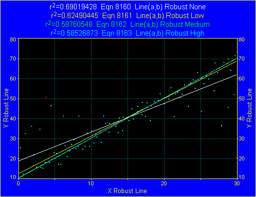
The least-squares straight-line curve-fit (white curve) clearly reveals the impact of outliers which significantly shift the fitted curve away from the bulk of the data. In this data set there are only two points outside 3 standard deviations and similarly only two between 2 and 3 standard deviations. When these four points are excluded and the data is refitted, the curve shifts somewhat closer to the bulk of the data.
Still, there is a sense that it is "likely" the curve should shift a great deal more toward the bulk of the data. What we should like then is a method that automatically offers a more robust fit, one that is far less sensitive to data points which are unlikely to be valid. With least squares, points less likely to be valid factor into the fit far more than those likely to be more accurate. TableCurve 2D’s non-linear engine offers exactly this type of robust or maximum likelihood fitting.
Three Optional Robust Procedures
TableCurve 2D’s non-linear fitting offers three robust methods that can be used instead of least squares. These methods are built directly into the non-linear engine enabling all non-linear functions, including UDFs and external C/Fortran functions, to be fitted by a robust method. The following graphs reflect the improvement realized by these three robust methods. In these examples, no points have been excluded from the fitting.
The Robust Low curve-fit (yellow reference) shows the improvement realized by least absolute deviation fitting. The Robust Medium curve-fit (green reference) is for the Lorentzian minimization, and the Robust High (blue reference) is for a robust procedure using the limiting form of the Pearson VII function. All three methods are more effective in offering the most likely fit, that which includes the bulk of the data. In the latter two, note that outliers are essentially ignored as they minimally influence the fit.
By selecting a robust minimization procedure in the Curve Fit Preferences option or within the separate customization dialogs for the Curve-Fit Peak Functions, the Curve-Fit Transition Functions, or the Curve-Fit Kinetic Equations option, robust fitting can be done for any of TableCurve 2D’s non-linear equations, including UDFs.
The Process menu also includes a Curve-Fit Robust Straight Line option which fits the simple straight line by least squares and by all three of TableCurve 2D’s robust minimizations.
When to Use Robust Methods
There are two instances where a robust method is particularly attractive. The first is the case shown in the above example where significant outliers are present and whose presence is adversely affecting the fitted curve. The other instance is when the y-data spans more than several orders of magnitude. As mentioned in the previous section, the squared residuals of the largest valued y-points can overwhelm the influence of the squared residuals of the smallest y-valued points, causing the smallest y-value points to either be poorly fitted or not fitted at all. Data that requires a logarithmic Y-scale to see all of the points may be a good candidate for robust fitting, especially if four or more major log divisions are present.
Least Absolute Deviation
The essence of robust fitting is to use a minimization that is less influenced by outliers and the dynamic range of the Y-variable. Instead of minimizing the sum of the squares of the residuals, an obvious alternative is to minimize the sum of the absolute value of the residuals:
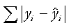
This is probably the best known robust method, though not necessarily the best, and is usually designated as least absolute deviation. Of TableCurve 2D’s three robust methods, least absolute deviation is the least powerful in terms of managing outliers.
Lorentzian Minimization
The intermediate method in terms of power of robustness is a Lorentzian minimization. Here what is actually being minimized is:
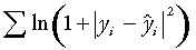
If you are uncertain of which robust method to use, we strongly recommend this Lorentzian minimization. It is very effective when you have noisy data with outliers or if your data spans many orders of magnitude in Y. These fits also tend to converge as rapidly as the least absolute deviation minimization.
Pearson Minimization
This is the most robust of the three methods. Here the minimization is:
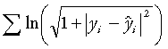
With this method, outliers tend to have almost no impact on the fitted curve. This minimization represents an extreme one where wild and random errors are expected as a natural course.
Gaussian Error Distribution
Each of the various minimization formulas corresponds with a maximum likelihood probability distribution. For least squares, this corresponding error distribution is Gaussian or normal. Relative to fit standard error (SE), a least squares goodness of fit, 95.4% of the data points should have residuals with a magnitude less than 2 SE (1 in 21.98 points should lay outside 2 SE). The value is 99.73% for residuals within 3 SE (1 in 370.4 points should lay outside 3 SE). The Gaussian distribution decays very rapidly. It suggests that only 1 of 15787 points should lay outside 4 SE, only 1 of 1.74 million points should lay outside of 5 SE, and those outside 6 SE should be only 1 in a half billion. In the real world where data is subject to human error, it is generally agreed that major errors are more likely or probable than the Gaussian distribution suggests.
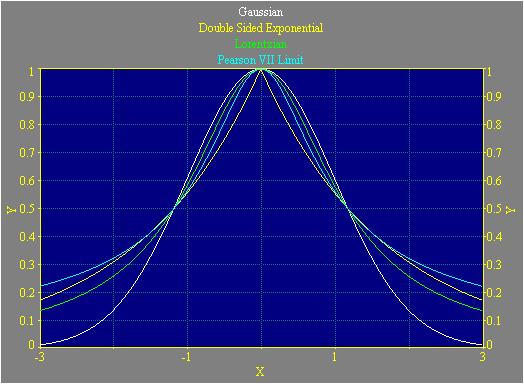
The following graph plots the error distributions. These are normalized so that amplitudes and FWHM (half-maximum widths) are equal.
Double Sided Exponential Error Distribution
The least absolute deviation fitting corresponds with a double-sided exponential probability distribution. While such a distribution produces reasonably wide tails, it also has a discontinuous first derivative at the peak center. As such, the actual error profile isn't likely to match this double-sided exponential in this center region. The tails of the double-sided exponential may however, be very practical.
This distribution suggests that 75.7% of the points should be within 2 SE and 88.0% within 3 SE. This distribution expects 1 of 16.9 points to be outside 4 SE, 1 of 34.3 to be outside 5 SE, and 1 of 69.6 to be outside of 6 SE. It is important here to recognize that such SE-relative values are based upon a least squares goodness of fit standard deviation.
Lorentzian Error Distribution
The Lorentzian minimization is strongly recommended for data with significant outliers because the Lorentzian distribution is a very natural one both at the center and the very wide tails. Such broad tails in effect state that significant errors are expected or likely and that points with such errors should minimally influence the fit.
The Lorentzian distribution suggests that 68.5% of the points should be within 2 SE and 83.3% within 3 SE. In terms of outliers, the Lorentzian expects 1 of 7.9 points to be outside of 4 SE, 1 of 9.8 to be outside of 5 SE, and 1 of 11.4 to be outside of 6 SE. Even out to 10 SE, the Lorentzian contains only 94.9% of the points, less than the Gaussian contains within 2 SE.
Pearson VII Limit Distribution
TableCurve 2D also offers a distribution with the same naturalness about the peak center as the Lorentzian but with extremely wide tails. This is based upon the Pearson VII function with a power term of 0.5. This is the smallest power term that can be used in the Pearson VII function and still have the peak converge to a finite area.
It is difficult to estimate areas for this distribution since area convergence does not occur until near infinity. If you know your model is very appropriate to your data, but that there is a high likelihood that a significant number of the data points are very seriously in error or perhaps even fabricated, this highly robust method may be a good choice for removing the impact of such points.
Analysis of Residuals
 The Display Residual Distribution format for the Residuals Graph displays a histogram of the residuals. Distributions with obvious asymmetry or wide tails would readily disqualify this assumption of Gaussian errors.
 The Display Residuals in Stabilized Normal Probability Plot format for the Residuals Graph is the preferred approach in TableCurve 2D for assuring errors are normal. A stabilized normal probability (SNP) plot uses an arcsine transformation on both X and Y to produce a normal probability plot that uses a linear scale for both the X and Y axes. On such a plot, perfectly normal errors plot as a 45 degree line. Critical limits also have a 45 degree slope, and lay equally above and below this line. TableCurve 2D modifies the SNP slightly and uses a delta SNP, where the X value is subtracted from the Y. This produces a horizontal y=0 for pure normal data, and horizontal critical limit lines.
TableCurve 2D plots 90, 95, 99, and 99.9% critical limit lines on the SNP plot. A 99% critical limit means that in only 1 out of 100 data sets should even a single point violate this limit. You may find the 99% critical limit the most useful. If even a single data point in the SNP violates this 99% limit, it is reasonable to assume that the errors fail this normality test. The following graph is from a curve fit which yielded normal errors.
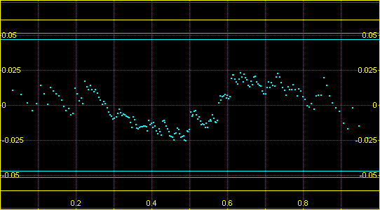
By default, the 90% critical limit lines will be blue, the 95% green, the 99% yellow, and the 99.9% red. You should inspect the SNP before attempting to use the parameter confidence statistics or confidence or prediction intervals in any way.
 The Error Models option in the Residuals Graph performs non-linear least-squares fits for the four error models and furnishes an r² value for each.
You should not assume simply because a distribution of errors is fitted well by a Gaussian that a robust procedure is if no value. Two key reasons for using a robust minimization are to deal effectively with outliers and a wide dynamic range on the Y-variable. It is very possible that such conditions will not be reflected in the fit of the overall residuals distribution.
Evenness of Residuals Distribution
In the noisy line example, the residuals are not evenly distributed across the X-range of the data. The errors at one end or in one region of the X-range have one sign and those at the other end or in another region have the opposite sign. In such cases, a more robust method may be desirable to lessen the impact of this uneven distribution of residuals.
Using Least-Squares
If the Y-range spans no more than a few orders of magnitude, there are no obvious outliers, and the errors appear to be normally distributed, you should use least-squares minimization. Most distributions in nature tend toward the Gaussian, and least-squares is perfectly sufficient most of the time. You should bear in mind that the robust methods do not have the same dynamic for convergence, and additional iterations and lengthier fits will be the price paid for utilizing one of the robust methods. Note that it may be necessary to set the maximum iterations to a higher count to insure convergence.
Non-Linear Nature of Robust Minimization
Whereas a non-linear iterative procedure is required in least-squares fitting whenever coefficients appear non-linearly in the equation, a non-linear procedure is always required for robust fitting. This means that the robust fitting of even the simple straight line equation must be done non-linearly. The Curve-Fit Robust Straight Line option in the Process menu uses the non-linear fitting engine with all four minimizations to fit the simple line equation. Although it is not necessary to fit the least squares minimization non-linearly, this is done simply to be consistent with the three robust minimizations which do require this non-linear fit.
Fitting a Linear Equation by a Robust Procedure
To fit any linear equation by a robust procedure, it must be fit non-linearly. For this reason there is now a Save TableCurve UDF option in the Review which will create a UDF for any of TableCurve 2D’s linear equations having ten or fewer terms, excepting the Chebyshev and Fourier series models. Such a generated UDF can then be fitted with a robust method as specified in the Curve Fit Preferences option.
Curve-Fit Statistics
To maintain a true basis for comparing the linear and non-linear equations in TableCurve 2D, all goodness of fit statistics are based upon sum-of-squares, even when a fit is made using a robust method. The r², DOF adjusted r², Fit Standard Error, and F-statistic are all based upon the sum of squared residuals. Even though a robust fit does not involve a least squares minimization, a sum of squared residuals is still computed in order to generate these numeric indices of fit.
The computation of standard errors and confidence ranges, as well as prediction and confidence intervals, are also based upon sum-of-squares computations and can be assumed accurate only when the residuals are normally distributed. If a chosen critical limit in the SNP is violated, or if the residuals distribution has narrower or wider tails than the Gaussian, or has appreciable asymmetry, then this assumption of normality fails, and these statistics should not be used as absolute measures of uncertainty. This is true for both least-squares and robust minimizations.
Graphical Inspection
Because these goodness of fit statistics for a robust minimization use a least squares measure, and no least squares optimization occurs, it is certain that these goodness of fit values will be inferior to those produced for the actual least squares fit. In many cases, the statistics for a robust fit will approach that of the least squares fit but they will never equal it. Thus in the option that fits a straight line by all four minimizations, the least squares case will always be at the top of the list, although any or all of the robust fits may be superior in being less influenced by outliers or in managing a wide dynamic Y range. This is simply one more reason to rely on graphical inspection as to the value of a robust fit. The instances where a robust fit is less influenced by outliers or where it fully manages a wide dynamic range in Y will not be apparent from the numeric indices of fit. Graphical inspection is essential.