Numerical Methods

Linear Fitting

All TableCurve 2D linear fitting algorithms except the high precision polynomials and rationals use 80 bit floating point math. This is the full 19-digit precision of Intel floating point units. This highest precision was chosen because most matrix operations are highly susceptible to precision losses and roundoff errors. Using software other than TableCurve 2D, even with the same procedures, you may find different fitted coefficient values for a given equation if such programs use 32 or 64 bit precision.

All of TableCurve 2D’s linearly fitted equation use a single step matrix solution method for the coefficients and a single step matrix inversion for the standard errors and confidence intervals.

The default (Fast Std) linear fitting procedures are as follows:

Equations Coefficients Errors/Confidence Intvls

1-2000 Direct Matrix Solution LU Decomposition

2001-8000 exc. high prec Gaussian Elimination LU Decomposition

High Precision Poly/Ratl Gaussian Elimination* Gauss-Jordan*

*The high precision polynomials and rationals use a 38-digit precision math emulator and special matrix routines which implement this higher precision floating point.

Optionally, for all except the high precision fits, a single method can be selected for resolving the coefficients, standard errors, and confidence intervals. The options include the Gauss-Jordan, LU-Decomposition (LU), and Singular Value Decomposition (SVD) procedures.

In a simple equation, the direct matrix, Gaussian Elimination, Gauss-Jordan, LU Decomposition, and Singular Value Decomposition methods are likely to produce identical coefficient values. As such, TableCurve 2D’s default uses the fastest methods for its simpler equations.

A separate set of built-in procedures, Fast SVD, is available where the SVD algorithm is used for fitting the standard precision 6000 series polynomial equations and the 7000 series rational equations. Higher order polynomials and rationals tend to have an ill-conditioned design matrix, exactly the type of situation where the SVD procedure can sometimes produce more stable results.

The SVD procedure manages ill-conditioning by pushing the coefficients closer to zero rather than the delicate balance offered by the other methods where the coefficients are driven toward very large positive and negative offsetting values. With higher order polynomials and rationals, the SVD procedure often produces unexpected though more stable coefficient values. The price for the added stability the SVD method offers is a reduced goodness of fit. Also, SVD requires almost an order of magnitude more fitting time than the other methods.

For more information on linear fitting algorithms, the following references may be of interest:

Bevington, Philip R. 1969, Data Reduction and Error Analysis for the Physical Sciences (New York: McGraw Hill)

Dongara, J.J. et al. 1979, LINPACK User’s Guide (Philadelphia: Society for Industrial and Applied Mathematics)

Press, William H. et al. 1992, Numerical Recipes in C; The Art of Scientific Computing (Cambridge,UK: Cambridge University Press)

Non-Linear Fitting

Non-linear equations cannot be solved in a single step solution of a matrix, but must be managed in an iterative fashion. As such, non-linear fitting is a much slower process and one that often requires starting estimates in order to initiate the fitting.

TableCurve 2D’s non-linear fitting engine is a 80-bit Levenburg- Marquardt algorithm that uses the Gauss-Jordan procedure for the matrix inverse required in each iteration. In non-linear fitting, the parameters are iteratively adjusted to minimize a goodness of fit merit function. If the algorithm is fully successful, a true global minimum is achieved.

When fitting any equation using a robust minimization, a non-linear iterative method is required even if the equation is a linear one. TableCurve 2D employs its own custom modifications of the Levenburg-Marquardt algorithm to enable three powerful robust minimizations in addition to least squares. These robust methods are explained in Chapter 11.

Since the Levenburg-Marquardt method’s minimization procedure requires the partial derivatives with respect to the parameters, TableCurve 2D uses analytic derivatives for the built-in non-linear functions for the highest precision and the most rapid fitting and convergence.

The Levenburg-Marquardt algorithm also requires starting estimates for the adjustable parameters. For the built-in non-linear equations, these are automatically supplied using pre-scan values specific to the current data profile.

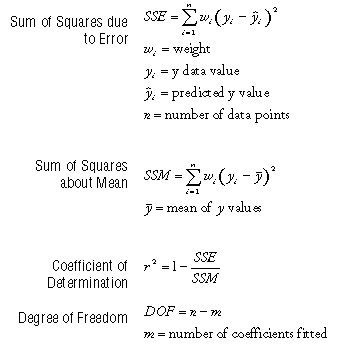
The non-linear fitting algorithm can be configured for the maximum number of iterations as well as to specify a convergence criteria. TableCurve 2D deems the algorithm converged when the r2 coefficient of determination is unchanging in the significant digit specified for five consecutive iterations. The fitting engine can also be interrupted to abort a non-linear fit that is going nowhere, but is still slowly changing in the r2 value.

TableCurve 2D’s fifteen user-defined functions are a part of the non-linear fitting engine. Here the starting estimates must be supplied by the user. User-functions are compiled and fitted in 80 bit precision, using numeric derivatives. Successful convergence may well depend upon the quality of the starting estimates.

Similarly, the up to 100 TCEX.DLL FORTRAN/C external functions are fitted using access points into the non-linear fitting engine.

For more information on the Levenburg-Marquardt non-linear fitting algorithm, see the Bevington and Press references previously given.

Integration, Minimization, And Root-Finding

TableCurve 2D uses the Gaussian Quadrature method for the main integration of the fitted equations and for cumulative areas. The Quadrature procedure’s convergence is targeted for eight significant figures. In the Evaluation option, the precision actually achieved is reported.

In the AI() and AIP() integration functions used in UDFs, a Gaussian Quadrature procedure is first used. If the target precision is not achieved, a Romberg procedure is then attempted. If neither algorithm achieves the target precision, the UDF will use the value from the procedure that came closest.

Brent’s method is used for determining the minima and maxima of the fitted equation and its derivatives. A partition approach is used to limit the possibility of reporting local minima.

The root-finding routine in TableCurve 2D and in its generated code is a multi-partition bisection procedure.

The roots of rational denominators are found using an eigenvalue procedure.

For more information on these methods, please refer to the Bevington and Press references.

Statistical