Autoregressive Modeling

AR estimation algorithms are used in the AR Modeling and Prediction option.

Autoregression

In an AR model, a value at time t is based upon a linear combination of prior values (forward prediction), upon a combination of subsequent values (backward prediction), or both (forward-backward prediction). The linear models give rise to rapid and robust computations.

AR Definitions

To preserve the degrees of freedom for statistical tests and to furnish a common reference for all AR algorithms, TableCurve 2D defines an AR model as follows:

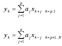
In these equations x is the data series of length N and a is the autoregressive parameter array of order p. TableCurve 2D uses the positive sign (linear prediction) convention for the AR coefficients. The model is defined as reverse prediction for the first p values, and forward prediction for the remaining N-p values. This definition is used for all AR fit statistics, although it is not the model fitted in any of the AR linear least-squares procedures.

Classes of AR Algorithms

The AR coefficients can be computed in a variety of ways. The coefficients can be computed from autocorrelation estimates, from partial autocorrelation (reflection) coefficients, and from least-squares matrix procedures. Further, an AR model using the autocorrelation method will depend on the truncation threshold (maximum lag) used to compute the correlations. The partial autocorrelation method will depend on the specific definition for the reflection coefficient. The least-squares methods will also yield results that are a function of how data are treated at the bounds (matrix size) as well as whether the data matrix or normal equations are fitted.

The AR algorithms in TableCurve 2D are least-squares procedures since these produce the best fits. Least-squares methods that offer in-situ separation of signal and noise through singular value decomposition (SVD) are the most robust of TableCurve 2D’s AR methods. These algorithms are built into the AR procedures (there is, for example, no separate Principal Component AutoRegressive or PCAR option).

AR Prediction Models

A continuous function of time needs only the computed parameters of the model to produce an estimate for any value of time desired. Whether the original time sampling is uniform or irregular is not a factor once the model is generated. This is not true for an autoregressive model. An AR linear prediction model is a discrete function that requires uniformly sampled data.

When an AR model is evaluated in the time domain for a future predicted value, the last portion of the data sequence is filtered by the AR coefficients to generate a new element. Although an AR linear prediction model does not explicitly contain a noise component, this is intrinsically a part of the data sequence. White noise is thus managed, provided it is uncorrelated, point to point.

AR Model Limitations

In practice, it may not be possible to predict a present value from past values. The process may be stochastic (truly random) rather than deterministic. There may be no correlation between past values and the current one.

Nor is the background noise necessarily white and uncorrelated. Geophysical processes, for example, are often characterized by red noise backgrounds. For red noise, the variance decreases with increasing frequency. In some cases, the overall noise trend can be approximated by a first order AR model.

As an AR model order increases, more of the trends in the data series are incorporated. When noise is completely absent, pure harmonics are captured with an order equal to twice the number of components. More commonly, though, some level of noise is present.

Further, the narrowband signals are often anharmonic. The signal components will be close to harmonic, evidencing regular oscillations, but cannot be described by a single sinusoid or exponentially-damped sinusoid. The information necessary to describe the oscillatory trend may require that the AR model capture several cycles of the oscillation. For slowly changing patterns, this can mean appreciable model orders.

AR Signal-Noise Separation

A basic AR model fit does not offer effective signal-noise partitioning. Even if pure sinusoids are embedded in modest levels of noise, it may require an order well beyond twice the signal component count to successfully capture and spectrally render the sinusoids. In other words, if a model order is too low, only a portion of the deterministic signal is captured. The remainder is treated as part of the white noise. Spectral components are thus missed.

On the other hand, if a model order is too high, the full deterministic signal is captured but some measure of the noise is also modeled. Spurious spectral peaks can result.

There are three ways to manage this limitation. First, the noise can be filtered or removed prior to analysis. Second, an optimum AR order can be selected that captures all of the deterministic signal elements and includes as little noise as possible. The third option consists of an in-situ noise removal within the least-squares procedures that generate the coefficients.

Model Order Determination

TableCurve 2D includes an AR Order Selection Criteria option to view normalized graphs of the MDL (Minimum Descriptive Length) and AIC (Akaike Information Criterion), the two indices most commonly used to determine optimum AR order. The minima in these criteria are the recommended model orders. These indices reflect major thresholds where increasing model order results in significant improvements in the AR fit. In general, though, these criteria are of limited use. Inappropriate model orders are sometimes suggested.

Signal Eigenmode Selection

Rather than struggle to find an optimum model order, an explicit signal-noise separation can be made. As the AR order increases, there are more coefficients to map both data trends and noise. If a matrix procedure based upon principal components is then used, the initial eigenvectors will describe only the signal components. The latter eigenvectors will capture the noise contributions. Model order is then less important, since the noise vectors are discarded prior to the computation of the AR coefficients.

This in-situ signal-noise separation is accomplished using singular value decomposition (SVD) in any of the least-squares AR models. The Graphically Select Signal and Noise Subspaces button is found in the AR Modeling and Prediction procedure. A visual indication of the signal-noise threshold is often given as the last major transition prior to a long sloping noise floor. Eigenmodes that capture an oscillatory signal component usually occur in close-to-equal magnitude pairs followed by a descending transition.

In the case of white noise, this type of visual eigenspace signal-noise separation is often successful even to levels where the noise power approaches that of the signal. The S/N range where this visual transition is apparent is not as great, however, in the case of red noise.

Complex Root Inspection

There is merit in exploring the complex roots of the AR model coefficients. The Plot Roots option will display the poles in either a unit circle or magnitude plot. Roots closest to the unit circle are usually indicative of signal, and those more to the interior are generally due to noise. This is another tool to assist in signal component determination.