Local Regression Spline Estimation

The Local Regression Spline Estimation option in the Estimate menu or the Process toolbar offers an adjustable order Loess-type (locally-weighted least-squares) procedure with two different weighting functions. This procedure combines Loess fitting, a discontinuous smoothing method, with the smoothness and continuity of a B-spline. This procedure can sometimes extract an underlying low frequency data pattern in extremely noisy data. This procedure is also useful for both upsampling and downsampling since the range and number of output points are specified. Uniform data are not required.

This option can be extremely slow and is not recommended for very large data sets.

The input data and local regression curve are shown in a TableCurve 2D Graph for rapid visualization of the effectiveness of the fit.

Algorithm

This procedure is a fitting and smoothing algorithm that performs a series of weighted least squares fits in a moving window across the data. The TableCurve 2D local regression estimation algorithm is similar to the Loess non-parametric estimation procedure. The TableCurve 2D algorithm also offers a Gaussian weighting function in addition to the tricube weighting function used in Loess. It also offers variable order fitting, from linear through quartic. For more information on the Loess algorithm, you may wish to refer to William S. Cleveland, "Visualizing Data", 1993, Hobart Press, Summit, NJ, ISBN 0-9634884-0-6.

Weighting Function

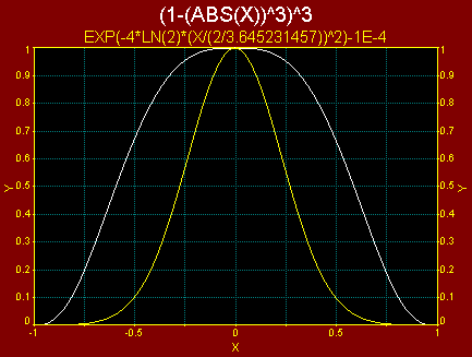
The tricube weighting function gives a much greater weight to nearby points as compared to a Gaussian. The following graph depicts both the tricube function and the particular form of Gaussian TableCurve 2D implements for this algorithm:

Model

You can choose to locally fit a linear (order 1), quadratic (order 2), cubic (order 3), or quartic (order 4) model to the data.

Data Window

The window minimum value incurs the minimum of smoothing. Higher window counts can be used to increasingly smooth the data.

Sectioning Data

You may enable or disable regions of data or individual points just as within TableCurve 2D's main Section Data option. When the state of one or more points is changed, the local regression and B-spline interpolant is recomputed and the graph is updated.

B-Spline Order

This is discussed in the Spline Estimation option. Note that the B-Spline will exactly pass through the smoothed data.

Goodness of Fit Statistics

A standard error (SE) and r² are reported. This is based upon the raw data and final spline interpolant. These statistics are of limited use, since a zero smoothing level and B-spline produce a perfect fit of noisy data. They may, however, allow a comparison between a favorable estimation and your choice of a parametric fit.

Output

The principal output will interpolate the spline model or Function. It is also possible to directly evaluate the first or second derivative (1st Deriv, 2nd Deriv).

For derivatives, be very cautious with noisy data. A significant level of smoothing is generally needed to produce accurate derivatives. With noisy data, significant smoothing is essential for valid derivatives. The separate Savitzky-Golay Spline Estimation option is recommended for serious derivative evaluations.

A quadratic spline has a continuous first derivative. A cubic spline is smooth in the first derivative and continuous in the second derivative. A quartic spline is smooth in both first and second derivatives and continuous in the third derivative. If you need a smooth derivative, be sure you use a spline order two greater than the derivative desired.

For the output, the number of elements n are generated between x start and x end. Up to 65536 values can be generated. The starting and ending X values should be at or within the range of the input data. The default values will perform a 2x upsampling within the x range of the data.

List

The List Data option lists the index, time, and output in a three column table. The listing uses the TableCurve 2D text viewer facility.

Copy

The Copy Data to Clipboard option copies the time and output values to the clipboard. Formats include full precision binary (for spreadsheets such as Excel) and ASCII (for pasting into text editors).

Save

The Save Data to Disk option writes the time and output values to a supported file format. These formats include ASCII, Excel 97/2000, Excel 95, Lotus WK3, Lotus WK1, SPSS, or Systat.

Production Facility

The TableCurve 2D Automation facility allows unattended processing of large numbers of data sets. The data sets can be consolidated in an Excel file or acquired using a DLL. The graphs can be exported to an MS Word/RTF file, while the processed data can be exported to an Excel 95 or Excel 97/2000 file.

The Reset button restores the data to its state when first entering the procedure. If an Automation Session is in progress, the Reset button can be used to terminate the automated processing.

Residuals

The Residuals button opens a TableCurve 2D Graph containing the residuals from the spline fit. The residuals are the difference between the data and spline model. This option is not available for the spline procedures that exactly interpolate the data.

Evaluation

The Evaluation option offers the means to more extensively evaluate the spline model. The evaluation can be be direct, or the computation can consist of first or second derivatives, roots, or integrated areas. This option can be used to generate a table or file of any size using a generated X grid or by importing X data from supported file formats.

MS Word/RTF Export

The MS Word/RTF File Export option is used to save the current graphs to either an MS Word file or a portable RTF (Rich Text Format) file. The graph is inserted into the file as a Windows metafile.

Automatic Update

The List, Residuals, and Evaluation windows are automatically updated when any change is made to the algorithm's settings.

Updating the Data Table

When exiting this procedure with the OK button, an option will be presented to update TableCurve 2D's main data table with the estimated data.

If Background Thread Fitting is active, the fitting will be initiated as soon as the estimation is accepted and the data is rescanned.