PeakLab v2 Documentation Contents            R2N Software Home            R2N Software Support

Whittaker Baselines

Whittaker-Based Baseline Estimation

Whittaker fitting is the modern standard for baseline correction in high-resolution chromatography and spectroscopy (DAD, FID, Mass Spec). Unlike morphological filters (Rolling Ball, Convex Hull) which treat the signal as a physical shape, Whittaker methods treat the baseline as a penalized least squares problem.

The Mathematical Foundation

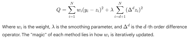
The Bohlmann-Whittaker algorithm seeks to find a baseline that minimizes a cost function balancing two competing goals:

Fidelity

How closely the baseline follows the original data.

Smoothness

How much the baseline resists rapid changes.

This is expressed via second-order finite differences:

In PeakLab, we utilize reweighted Whittaker algorithms, which apply a weight vector w to the fidelity term. This allows the algorithm to "ignore" positive peaks while staying pinned to the noise floor. These are iterative fitting algorithms.

Strengths and Applications

Noise Centering

Ideal for detectors where noise is centered around the baseline (e.g., UV-Vis, DAD).

Numerical Stability

Optimized via pentadiagonal matrix solvers, ensuring rapid convergence even for large datasets.

Flexibility

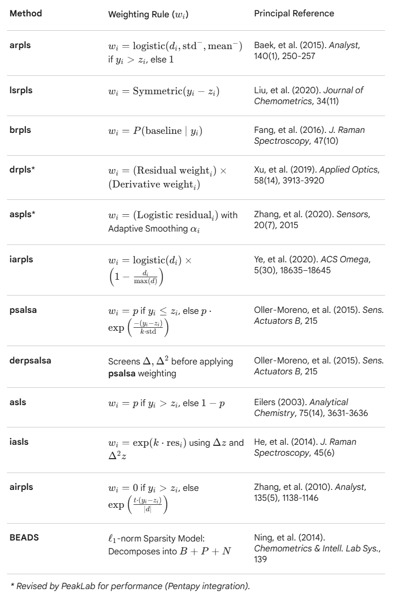
Different weighting schemes (arPLS, asPLS, drPLS) allow for varying levels of peak suppression and curvature adaptation.

Comparison: When to Use Whittaker vs. Morphological

Key References

     Bohlmann, G. (1899). Ein Ausgleichungsproblem. Nachrichten von der Königlichen Gesellschaft der Wissenschaften zu Göttingen, Mathematisch-physikalische Klasse.

     Whittaker, E. T. (1923). A new method of graduation. Proceedings of the Edinburgh Mathematical Society.

     Henderson, R. (1924). On a new method of graduation. Transactions of the Actuarial Society of America, 25, 29–40.

     Eilers, P. H. C. (2003). A Perfect Smoother. Analytical Chemistry, 75(14), 3631–3636. https://doi.org/10.1021/ac034173t.

     Eilers, P. H. C., & Boelens, H. F. M. (2005). Baseline correction with asymmetric least squares smoothing. Leiden University Medical Centre Report. [Unpublished technical report] (asLS)

     Baek, S.-J., Park, A., Ahn, Y.-J., & Choo, J. (2015). Baseline correction using asymmetrically reweighted penalized least squares smoothing. The Analyst, 140(1), 250–257. https://doi.org/10.1039/C4AN01061B (arPLS)

     Xu, D., Liu, S., Cai, Y., & Yang, C. (2019). Baseline correction method based on doubly reweighted penalized least squares. Applied Optics, 58(14), 3913–3920. https://doi.org/10.1364/AO.58.003913 (drPLS)

     Oller-Moreno, S., Pardo, A., Jiménez-Soto, J. M., Samitier, J., & Marco, S. (2014). Adaptive asymmetric least squares baseline estimation for analytical instruments. In 2014 IEEE 11th International Multi-Conference on Systems, Signals and Devices (SSD), 1–5. https://doi.org/10.1109/SSD.2014.6808837 (psalsa)

     Korepanov, V. I. (2020). Asymmetric least-squares baseline algorithm with peak screening for automatic processing of the Raman spectra. Journal of Raman Spectroscopy, 51(10), 2061–2066. https://doi.org/10.1002/jrs.5952 (derpsalsa)

     Zhang, F., Tang, X., Tong, A., Wang, B., Wang, J., Lv, Y., Tang, J., & Wang, J. (2020). Baseline correction for infrared spectra using adaptive smoothness parameter penalized least squares. Spectroscopy Letters, 53(3), 222–233. https://doi.org/10.1080/00387010.2020.1730908 (aspls)

     Askar, S. S., & Karawia, A. A. (2015). On solving pentadiagonal linear systems via transformations. Mathematical Problems in Engineering, 2015, Article 232456. https://doi.org/10.1155/2015/232456

     Müller, S. (2019). pentapy: A Python toolbox for pentadiagonal linear systems. Journal of Open Source Software, 4(42), 1759. https://doi.org/10.21105/joss.01759

     Erb, D. (2024). pybaselines [software], version 1.x. https://github.com/derb12/pybaselines (lsrpls, brpls)
 

Whittaker Parameter Tuning (lambda and p)

Most Whittaker-based routines (asls, arpls, airpls, etc.) rely on two primary variables that define the "stiffness" and "directionality" of the baseline.

Smoothness (lambda)

     Physical Meaning: The "Tension" of the baseline.

     High lambda: The baseline behaves like a rigid steel rod; it remains a straight line and ignores all fluctuations.

     Low lambda: The baseline behaves like a flexible string; it follows every curve and noise wiggle.

Asymmetry (p)

     Physical Meaning: The "Directional Bias".

     Definition: In algorithms like asls, p is the weight assigned to positive residuals (peaks) and 1-p is assigned to negative residuals (noise/valleys).

     The Value: Usually set very small (e.g., 0.001 to $0.01).

     Mechanism: By setting p low, the algorithm "penalizes" the baseline for going into a peak but allows it to stay centered within the noise floor.

     Note on 'arpls/iarpls': These use a self-tuning weighting function instead of a fixed p, but they still use lambda to define the overall stiffness.

Whittaker Algorithms

arpls - Asymmetrically Reweighted Penalized Least Squares

Iteratively suppresses positive residuals (peaks) more than negative ones to estimate a smooth baseline without being biased by signal peaks.

lsrpls - Locally Symmetric Reweighted Penalized Least Squares

Applies symmetric weighting to penalized least squares, improving baseline fit in symmetric peak regions.

brpls - Bayesian Reweighted Penalized Least Squares

Uses Bayesian modeling to estimate peak proportions and reweight the baseline fit.

drpls - Doubly Reweighted Penalized Least Squares

Applies two layers of reweighting to better suppress peaks and noise during baseline estimation.

aspls - Adaptive Smoothness Penalized Least Squares

Dynamically adjusts the smoothing parameter across the signal to better handle variable baseline curvature.

iarpls - Improved Asymmetrically Reweighted Penalized Least Squares

Enhances arpls by refining the weighting scheme for better convergence and peak suppression.

psalsa - Peaked Signal's Asymmetric Least Squares Algorithm

Like asls but uses exponential decay weighting for values above the baseline, allowing better handling of noisy, peak-heavy data.

derpsalsa - Derivative Peak-Screening Asymmetric Least Squares Algorithm

Enhances psalsa by screening peaks using smoothed first and second derivatives before reweighting.

asls - Asymmetric Least Squares Smoothing

Classic baseline method that penalizes positive residuals more than negative ones to suppress peak.

iasls - Improved Asymmetric Least Squares Smoothing

Extends asls by incorporating both first and second derivatives of residuals.

airpls - Adaptive Iteratively Reweighted Penalized Least Squares

Iteratively updates weights based on residuals, adaptively suppressing peaks and improving convergence.

Manual Parameter Adjustment for Whittaker Algorithms

The Whittaker-based baseline algorithms are highly effective, but manually adjusting their parameters can feel counterintuitive. This is primarily because the required smoothing stiffness is heavily dependent on the number of data points (N) in your spectrum.

The Smoothing Penalty (lambda)

Lambda controls the "stiffness" or rigidity of the fitted baseline. Because the algorithm calculates differences between adjacent data points, a higher data density requires a dramatically higher lambda to achieve the same visual stiffness.

Starting Heuristic: A highly reliable starting point is to set Lambda somewhere between N^1.5 (for a more fluid, flexible baseline that tracks local minima) and N^2 (for a rigid, stiffer baseline).

Magnitudes: Depending on your data density, do not be surprised if lambda requires values in the hundreds of thousands or millions (e.g., 10^5 to 10^7). Furthermore, "loose" algorithms like airPLS naturally require much higher Lambda values to prevent the baseline from creating wild excursions into the peaks.

The Asymmetry Weight (p)

For algorithms that utilize the p parameter (such as asls, psalsa, and aspls), this value dictates the baseline's tendency to stay beneath the data.

Starting Heuristic: Set this parameter to a value very close to zero, typically between 0.001 and 0.05.

Behavior: A value of 0.01 heavily penalizes the baseline for rising above the data, forcing it to cleanly "hug" the noise floor and minimizing the number of points that fall below the baseline. Increasing the p value relaxes this penalty, which will shift the entire baseline upward in the y-dimension.

Whittaker Algorithm Optimization to Match Human Designed Baselines

The easiest way to determine the proper lambda and p for the Whittaker algorithms and the frequency cutoff, the three lambdas, and the asymmetry for the BEADS is to use the Baseline procedure's option for Optimization.

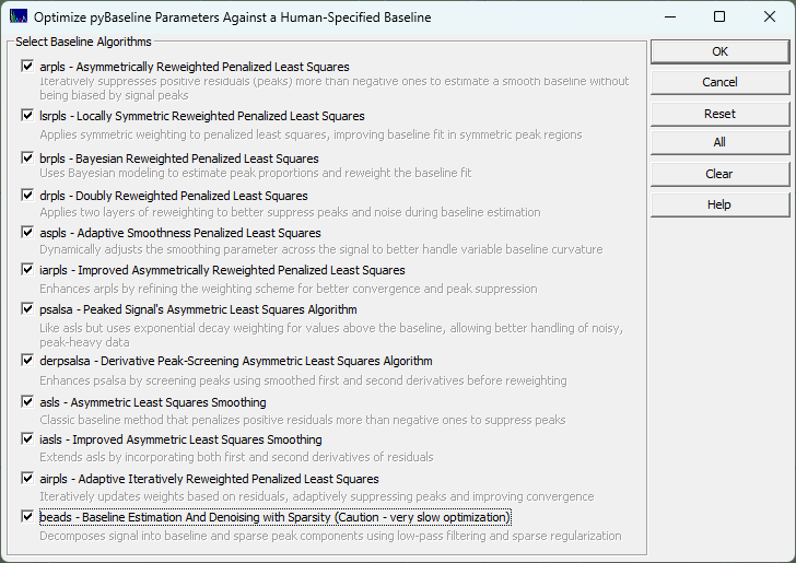
The best way to determine which algorithm to use, we suggest you use the human element. In the Baseline procedure, you will see an Optimize button that opens the above dialog. We recommend you use the SD Variation for the Baseline Detection and the Non-Parm Linear for the Model.

To save time, adjust the automatic settings to get the baseline reasonably close, and then using the mouse highlight and unhighlight the baseline and peak regions until to the human eye you have what you perceive as the perfect human designed baseline baseline. You will probably want to set the non-parametric points to the minimum of 3 if you have very small zones of baseline resolved zones to work with.

Once you have created the optimum human-designed baseline as in the example above, it is recommended that you save your manual baseline for future use in similar data sets, or as a starting point for future optimizations.

Do not make any changes in the dialog settings. If you do, the automated algorithms will re-estimate or re-fit the baseline points. Because of the amount of effort to create a human baseline, it is recommended that you save the baseline after creating it. Right click the graph of the human baseline after it is complete for these save options:

Save this Baseline/Non-Baseline State

Use this option to save an ASCII CSV containing this baseline state information. This can be subsequently imported to recreate the zones in time that you have specified as baseline in any data set irrespective of its x range or sampling rate.

Import this Data Set's Baseline/Non-Baseline State
Import All Data Sets' Baseline/Non-Baseline State

These options import the saved baseline state information for the current data, or for all data sets currently loaded.

Save this Baseline as an XY File

You can also save the actual baseline curve as an XY file. This will save the actual fitted baseline (the while line in the sample), at the x values in the data set.

Import this Data Set's Baseline from XY File

This option will import the XY fitted baseline and apply it to the current data set.
 
After optionally saving your human target upon which the optimizations are to train, click the Optimize button. You must leave the algorithm set for the non-parametric model or whatever model was used to construct the human baseline.

Only when you have the best human-engineered baseline you can devise, click the Optimize button. Select the algorithms you wish to train to match your human baseline. Click OK to initiate a set of generic algorithm (differential evolution) optimizations where the parameter(s) of each Whittaker algorithm are optimized to match as closely as possible your human designed baseline. PeakLab launches an embedded python procedure to perform these training optimizations.

Note that you are training these algorithms how to process just this specific type of separation or spectral analyses. Baselines of an entirely different rate of change or data with significantly different S/N, sampling rate, or width of peaks will require separate optimizations.

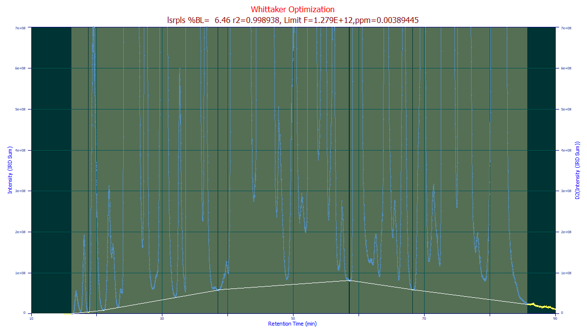
When the optimizations are complete, you will see a summary similar to the following:

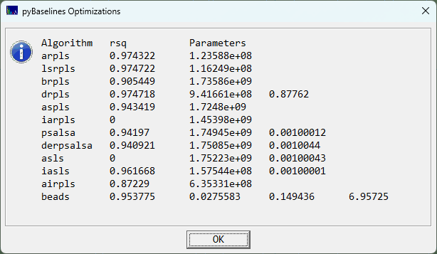
In this example, the arpls, lsrpls, and drpls outperformed the other algorithms in matching the human designed baseline. When you click OK, the parameter(s) for each of the algorithms will be automatically updated in the dialog so that you can view the optimizations.

Choose the Partial option each time it appears if you want to keep the human designed baseline points displayed. Note that these points are only used for the opitmization. The Whittaker baselines algorithms override your selected points as each determines it own set of peaks and baseline points in the data. The genetic algorithm simply finds the parameters that best match your human designed baseline using its own internal methodology for separation peaks and baseline. Again, your own specified points are not used once the optimization are complete, even if you choose to have them displayed as a reference.

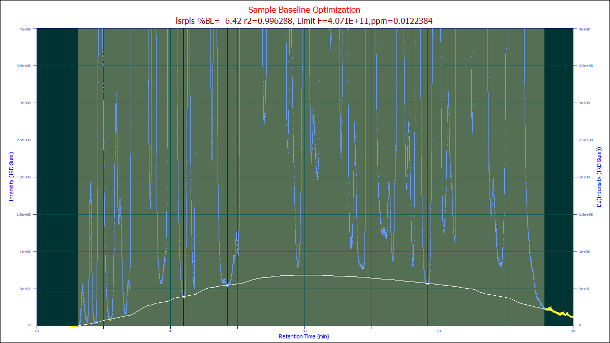
If the arpls algorithm is chosen as the Model after this optimization, the optimized arpls lambda will be used, generating the white baseline above. You can then select all of the different baselines in you wish to see which one best manages your specific baseline.

BEADS and XPS Baseline Algorithms

The BEADS and XPS baseline algorithms are non-Whittaker algorithms that are also offered in the Baseline option. Please be wary of optimizing the BEADS algorithm alongside the Whittaker algorithms. BEADS is notoriously hard to manually tune, and as such the optimization may be of appreciable value, but it is a computationally expensive iterative algorithm and the GA must optimize five different parameters.